

Overview › Build it in GraphPad Prism › Guide 6
Alternating treatments, multielement, and changing criterion
These designs use the same Prism graph you already know. Each needs one or two extra settings: keeping each condition’s points connected across blank rows, giving each condition its own symbol and a legend, or adding dashed criterion lines.
You will be able to
- Keep each condition’s points connected across blank rows in an alternating treatments or multielement graph, and give each condition a symbol that can be told apart in black and white.
- Make a legend inside the plot that lists only the conditions a reader needs, in 10-point text.
- Add dashed criterion lines from a Criterion data set and label each subphase with its criterion in a changing criterion graph.
Your graph doesn’t need this guide. Guide 6 is for alternating treatments, multielement (functional analysis), and changing criterion graphs. The graph you chose, Reversal (ABAB), has none of these extra settings. Go on to Guide 7: Export and place the figure. If you haven’t yet, stack your tiers in Guide 5: Multiple baseline graphs, then go on to Guide 7: Export and place the figure. Building one of those graphs instead? Choose it in the Graph box above so every guide shows its steps, or go straight to its section: alternating treatments, multielement, or changing criterion.
Guides 3 and 4 already covered these steps for your graph. They walked you through each one with your practice data and pictures. This guide collects the settings and checks that are specific to each design in one place, so you can check your work or build the next graph from your own data. Your section: Alternating treatments design. Your section: Multielement design (functional analysis). Your section: Changing criterion design.
Alternating treatments design
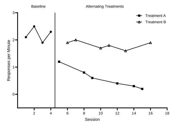
Practice data: practice-atd-data.xlsx, 16 sessions in A1:D17. Finished project: alternating-treatments.prism (or .pzfx for older versions).
Give each condition its own data set, just like a phase. During the alternating phase, each session’s value goes in the data set for the condition run that session. Each treatment’s data set then has blank cells between its values.
| X | A | B | C | |
|---|---|---|---|---|
| Title | Session | Baseline | Treatment A | Treatment B |
| 1–4 | 1–4 | 2.1 … 2.3 | ||
| 5 | 5 | 1.2 | ||
| 6 | 6 | 1.9 | ||
| 7 | 7 | 2.0 | ||
| 8 | 8 | 0.8 | ||
| 9 | 9 | 0.6 |
- Build the graph as usual. Make an XY table and paste the data as in Guide 1, and make a Points & connecting line graph as in Guide 2. Format it as in Guide 3, with rate settings on the vertical axis: Minimum -0.5, Maximum 3, Major ticks interval 1, and Starting at Y= 0. The practice rates peak at 2.5, so a maximum of 3 leaves room for the legend. Set the horizontal axis from 0 to 18, the first multiple of 2 past session 16, with an interval of 2 and Starting at X= 2, so session 0 has no number.
- Keep each condition connected across its blank rows. In Format Graph › Graph Settings, keep Connect adjacent points, Prism’s default, under For point-to-point connecting lines, at each missing or off-scale Y value. Each treatment is then one continuous path. The baseline path still stops at the phase change, because its data set has no later values to connect to.
- Give each condition a different symbol. In Format Graph › Appearance, choose each data set in the Data set list and pick its shape: filled circles for Baseline, filled squares for Treatment A, and open (hollow) triangles for Treatment B. Keep every symbol black at size 4, and every line black, solid, and 1 pt.
A treatment’s path breaks into pieces? Graph Settings is set to Leave a gap; choose Connect adjacent points. A path dips to zero between points? A cell that should be empty holds a 0. Select it in the data table and press Delete.
- Add the phase-change line and labels. Follow Guide 4. The practice data change phase once, after session 4, so the X axis gets one additional tick at 4.5 with Line ticked: solid black, 1 pt. Add two label ticks with Show Text on, Location Above, horizontal, an offset of 9.2 cm, and no tick or grid line: Baseline at 2.5 and Alternating Treatments at 10.5.
- Keep only the treatments in the legend. In Format Graph, choose Baseline in the Data set list and untick Show legend. Baseline is already named by its phase label. The legend then lists only Treatment A and Treatment B.
- Tidy the legend. Prism places the legend inside the plot, at the top right, once the axes have their custom lengths (if it doesn’t, drag it there). Each entry is its own object. Set each to 10 pt with the font size list on the Text toolbar, then select both and choose Arrange›Align Objects›Left. Make sure it covers no data and ends before the end of the X axis. Instead of a legend, you can also label each treatment’s path directly with the Text tool, near its last point.
Check your alternating treatments graph
- Treatment A and Treatment B are each one continuous path, connected across blank rows
- The Baseline path ends at session 4 and does not join either treatment
- Each condition has its own symbol: filled circles (Baseline), filled squares (Treatment A), open triangles (Treatment B)
- One solid phase-change line at 4.5, from the X axis to the top of the plot
- The labels Baseline and Alternating Treatments sit above the plot, centered over their phases, each on one line
- The legend inside the plot lists only Treatment A and Treatment B, in 10-pt text, and covers no data
- Vertical axis −0.5 to 3, interval 1, starting at 0, so the numbers are whole and zero floats half a tick above the X axis
Then read the graph. Do the two treatment paths separate clearly, with little or no overlap, across the whole alternating phase? See what experimental control looks like in an alternating treatments design.
Multielement design (functional analysis)
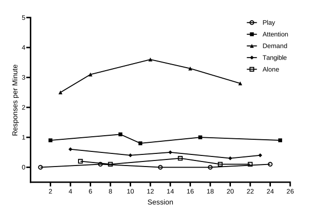
Practice data: practice-fa-data.xlsx, 25 sessions in A1:F26. Finished project: multielement-fa.prism (or .pzfx for older versions).
- One data set per condition. Put session numbers in X and one condition in each data set, A to E: Play, Attention, Demand, Tangible, and Alone. Each session’s rate goes under the condition run that session, so every row has exactly one rate. Type 0 for a session with no responding. Leave a cell blank only when that condition was not run in that session.
| X | A | B | C | D | E | |
|---|---|---|---|---|---|---|
| Title | Session | Play | Attention | Demand | Tangible | Alone |
| 1 | 1 | 0 | ||||
| 2 | 2 | 0.9 | ||||
| 3 | 3 | 2.5 | ||||
| 4 | 4 | 0.6 | ||||
| 5 | 5 | 0.2 | ||||
| 6 | 6 | 3.1 | ||||
| 7 | 7 | 0.1 |
- Make and format the graph. Make a Points & connecting line graph and format it as in Guide 3. On the vertical axis, set Minimum -0.5, Maximum 5, Major ticks interval 1, and Starting at Y= 0. The practice rates peak at 3.6, so a maximum of 5 leaves room for the legend in the upper right. Set the horizontal axis from 0 to 26, one more than the last session, with an interval of 2 and Starting at X= 2.
- Keep each condition connected across its blank rows. Keep Connect adjacent points, Prism’s default, in Format Graph › Graph Settings. Every condition’s data set has blanks between its values, so with Leave a gap all five conditions would show as scattered points.
- Use five distinguishable symbols. The practice graph uses open circles for Play, filled squares for Attention, filled triangles for Demand, filled diamonds for Tangible, and open squares for Alone, all black at size 4. Open circles for the control (Play) condition is a common pattern. What matters most is that every symbol reads clearly in black and white and stays the same across all your figures.
- Skip the phase-change lines and phase labels. All five conditions alternate within one phase, so there is nothing to separate or name. The legend identifies the conditions instead.
- Keep and tidy the legend. Leave Show legend ticked for all five conditions. Prism places the legend inside the plot, at the top right, once the axes have their custom lengths (if it doesn’t, drag it there). Set each entry to 10 pt with the font size list on the Text toolbar, select all five, and choose Arrange›Align Objects›Left. Make sure it covers no data and ends before the end of the X axis. The legend lists the data sets in the order of the table’s columns, and the practice file puts the control condition, Play, first. To change the order, move the columns in your spreadsheet before you paste. Whatever order you choose, use it in every figure.
Zero rates stay visible. With the floating zero from Guide 3, sessions with no responding sit on the 0 line, just above the X axis, instead of on it. Keep symbols at size 4 or larger. When two conditions share a shape, as Attention and Alone do here, make one filled and the other open so they can still be told apart in black and white.
Check your multielement graph
- No phase-change lines and no phase labels
- Five paths, each connected across blank rows
- Five symbols that can be told apart in black and white
- The legend inside the plot lists Play, Attention, Demand, Tangible, and Alone, in 10-pt text, and covers no data
- Sessions with no responding are typed as 0 and sit on the 0 line, above the X axis
- Vertical axis −0.5 to 5, interval 1, starting at 0, so the numbers are whole and zero floats half a tick above the X axis
Then read the graph. Is responding in any test condition consistently higher than in the Play (control) condition, with little overlap? See Functional analysis: differentiated or not?
In the practice graph, Demand is clearly highest, at 2.5 to 3.6 responses per minute. Attention (0.8 to 1.1) and, at a lower level, Tangible (0.3 to 0.6) are also above Play (0 to 0.1) in all five cycles, with no overlap. Alone stays low (0.1 to 0.3) and overlaps Play at 0.1. Because each test condition is compared with Play, not just with the highest condition, this graph suggests escape plus attention, and possibly tangible: multiple control worth following up.
Changing criterion design
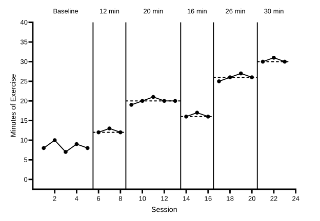
Practice data: practice-cc-data.xlsx, 23 sessions in A1:G24. Finished project: changing-criterion.prism (or .pzfx for older versions).
Why the subphases differ. The practice subphases last 3, 5, 3, 4, and 3 sessions, the criterion changes by different amounts (+8, −4, +10, and +4 minutes), and it steps back down from 20 to 16 minutes for a while. When behavior follows changes like these, time alone can’t explain them (see how the design shows control). The criterion rows work the same for any subphase lengths and criteria: each line spans exactly its own subphase.
- One data set per subphase. Title the data sets Baseline, Phase 1, Phase 2, Phase 3, Phase 4, and Phase 5 (A to F), so the data path breaks at every criterion change. Make the graph and format it as in Guide 3. On the vertical axis, set Minimum -2.5, Maximum 40, Major ticks interval 5, and Starting at Y= 0. The practice data peak at 31 minutes, so a maximum of 40 keeps the highest point well below the top of the plot. Set the horizontal axis from 0 to 24, one more than the last session, with an interval of 2 and Starting at X= 2.
- Add the phase-change lines. Follow Guide 4, Part A. The practice data change phase after sessions 5, 8, 13, 16, and 20, so the X axis gets additional ticks with Line ticked at 5.5, 8.5, 13.5, 16.5, and 20.5. Keep these lines solid.
- Type the criterion rows. In the next empty data set, G, type the title Criterion. Starting at row 24, just below the last session, type the X values and criterion levels below. Each criterion line is two rows, from half a session before its subphase’s first session to half a session after its last, at the criterion level. Leave the Criterion cell empty in the row between two lines.
| X | G | |
|---|---|---|
| Title | Session | Criterion |
| 24 | 5.5 | 12 |
| 25 | 8.5 | 12 |
| 26 | 8.5 | |
| 27 | 8.5 | 20 |
| 28 | 13.5 | 20 |
| 29 | 13.5 | |
| 30 | 13.5 | 16 |
| 31 | 16.5 | 16 |
| 32 | 16.5 | |
| 33 | 16.5 | 26 |
| 34 | 20.5 | 26 |
| 35 | 20.5 | |
| 36 | 20.5 | 30 |
| 37 | 23.5 | 30 |
- Make the criterion lines dashed. In Format Graph, choose Criterion in the Data set list. Untick Show symbols and Show legend, and set the connecting line to black, 1 pt, with a dashed Pattern. Dashing keeps the criterion visibly different from the data path and the solid phase-change lines.
- Break the path between criterion lines. On the Graph Settings tab, choose Leave a gap. Without it, Prism would join the end of each criterion line to the start of the next, across the empty row.
- Label each subphase with its criterion. Use the phase-label method from Guide 4, Part B: one tick per label with Show Text on, Location Above, horizontal, an offset of 9.2 cm, and no tick or grid line. The labels are Baseline at 3, then 12 min at 7, 20 min at 11, 16 min at 15, 26 min at 18.5, and 30 min at 22.01. The middle of the last subphase is session 22, which has a number under the axis, so its label is typed 0.01 aside.
Changed a criterion? Edit its two values in the Criterion data set and its label’s Text line 1. The dashed line and the label move with the numbers.
Check your changing criterion graph
- The data path breaks at every phase change
- Five solid phase-change lines at 5.5, 8.5, 13.5, 16.5, and 20.5, from the X axis to the top of the plot
- Five dashed criterion lines at 12, 20, 16, 26, and 30, each spanning only its own subphase
- The Criterion data set has no symbols and no legend entry, and Graph Settings is on Leave a gap
- The labels Baseline, 12 min, 20 min, 16 min, 26 min, and 30 min sit above the plot, centered over their subphases, and every number under the X axis still shows
- Vertical axis −2.5 to 40, interval 5, starting at 0, so zero floats half a tick above the X axis
Then read the graph. Does responding shift to each new criterion soon after it changes and stay near it until the next change? See what experimental control looks like in a changing criterion design.
Finished Prism projects for all three designs, with the connection settings, symbols, legends, criterion lines, and labels already in place, are on the templates page.