

Overview › Build it in GraphPad Prism › Guide 3
Format for APA style
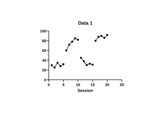
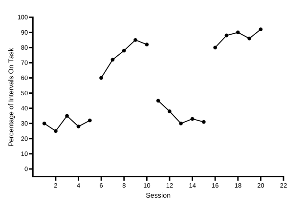
Two Prism dialogs do almost all of this guide’s work. Format Graph makes the symbols and lines black. Format Axes sets the graph’s size, the axis ranges with zero floating above the horizontal axis, the fonts, and the titles. Parts A and D each end with a picture of how your graph should look. You are formatting the Participant 1 graph. Guide 5 copies its formatting to the other tiers, so every setting you make here carries over. For your graph, Part A also gives each condition its own symbol and keeps each condition’s points connected across blank rows.
You will be able to
- Make every data set black with 1-pt lines and filled circles and a different symbol for each condition, connected across blank rows, and turn off the legend entries the graph doesn’t need.
- Set the graph’s size by its axis lengths, and set both axis ranges with zero floating half a tick above the horizontal axis and session 0 left unlabeled.
- Hide the graph title, set plain Arial fonts, and add axis titles that name the measure.
Two dialogs, several tabs. Format Graph opens when you double-click a data point, or from Change›Symbols & Lines. Its tabs are Appearance, Data Sets on Graph, and Graph Settings. Format Axes opens when you double-click an axis, or from Change › Frame and Origin, X Axis, or Y Axis (left). Its tabs are Frame and Origin, X axis, Left Y axis, Right Y axis, and Titles & Fonts. You can move between the tabs of an open dialog without closing it.
Part A: Make every data set black
- Open Format Graph. Double-click any data point, or choose Change›Symbols & Lines. The dialog opens on the Appearance tab.
- Change all the data sets at once. Open the Data set list at the top of the tab and choose --- Change ALL data sets ---, the first item. Every setting you make now applies to all four data sets.
- Set the symbols. Under Show symbols, set Color to black and Size to 4. In the Shape palette, choose the filled circle. You choose each condition’s shape in step 5. Prism measures symbols in steps of 1.44 pt, so size 4 is 5.76 pt across, the closest match to the 6-pt markers in the Excel lessons.
- Set the connecting lines. Under Show connecting line/curve, set Color to black, Thickness to 1 pt, and Pattern to solid, the first pattern in the list.
- Give each condition its own symbol. Choose one data set at a time in the Data set list and pick its shape in the Shape palette: Baseline 1 filled circles, Intervention 1 filled circles, Baseline 2 filled circles, and Intervention 2 filled circles. For an open symbol, choose the hollow version of the shape. Keep every symbol black at size 4: shape and fill, never color, tell the conditions apart.
- Turn off the legend.Turn off Baseline’s legend entry.Keep the legend. With --- Change ALL data sets --- still chosen, untick Show legend under Additional options. Every legend entry disappears. A single-case graph names its phases with labels above the plot, which you add in Guide 4. Choose Baseline in the Data set list and untick Show legend under Additional options. Leave it ticked for Treatment A and Treatment B: in the alternating phase, the legend is what tells them apart. The Baseline phase gets a label above the plot in Guide 4. Leave Show legend ticked for all five conditions. A multielement graph has no phases to label, so the legend is how a reader matches each path to its condition. Guide 4 tidies it.
- Keep each condition connected across blank rows. Click the Graph Settings tab. Under For point-to-point connecting lines, at each missing or off-scale Y value, keep Connect adjacent points, Prism’s default. That is what joins each condition’s points across the rows where another condition ran. Leave a gap would break every condition into short pieces. The Baseline path still ends at the phase change, because its data set has no values after session 4.
- Click OK and compare. Click OK to close Format Graph.
Part B: Set the size and the frame
- Open Format Axes on the Frame and Origin tab. Choose Change›Frame and Origin. Keep this dialog open through Part D, moving from tab to tab.
- Put the origin at the lower left. Set Set origin to Lower left.
- Set the axis lengths. Set Shape to Custom. Then set Width (Length of X axis) to 13.97 cm and Height (Length of Y axis) to 8.89 cm. If your Prism measures in inches, type 5.5 and 3.5. For now, build Participant 1’s tier at this full size. Guide 5 makes each tier shorter.
- Remove the frame. Set Frame style to No frame, so the graph has a plain X axis and Y axis and no box around the plot. Leave Thickness of axes on Auto; at this size Prism draws the axes about 1.5 pt thick. When the axes get their new lengths, Prism moves the legend inside the plot, at the top right. If it doesn’t, drag it there. Leave it for now; Guide 4 tidies it.
Why these lengths? In Prism, the axis lengths are the size of the plot itself, the space inside the axes. Graphing standards recommend a plot about two-thirds as tall as it is wide, and the accepted range runs from 5:8 to 3:4. Flatter graphs make changes look smaller, and taller ones make them look bigger. 8.89 cm is 0.64 of 13.97 cm, close to 2:3. With the numbers and titles around the plot, the whole graph comes out about 17 cm (6.7 in) wide, which fits a manuscript page (Guide 7). Set the size before the fonts: font sizes are fixed in points, so text you set now prints at that size.
Part C: Set the axis ranges and the floating zero
- Turn off the automatic range on the vertical axis. Click the Left Y axis tab and untick Automatically determine the range and interval.
- Set the range and the ticks. Type -5 in Minimum and 100 in Maximum. Type 10 in Major ticks interval and 0 in Starting at Y=. The minimum is half an interval below 0, and the numbered ticks start at 0. So zero floats half a tick above the horizontal axis, and no negative number shows. Your graph shows a rate, but an interval of 1 keeps the axis numbers whole (0, 1, 2, and so on); the points still plot at their exact rates. On this tab, also set Decimals to Auto (the option shows Auto with a number in brackets); if the numbers still show a decimal point, choose Integers. For your own data, end the vertical axis at 100 for percentages; for other measures, at a tick comfortably above your highest value, leaving room for the legend inside the plot. The practice data are percentages, so the maximum is 100. The practice rates peak at 2.5, so a maximum of 3 leaves room for the legend. The practice rates peak at 3.6, so a maximum of 5 leaves room for the legend. The practice data peak at 31 minutes, so a maximum of 40 keeps the highest point well below the top of the plot. Then set the minimum to minus half the interval.
- Set the horizontal axis. Click the X axis tab and untick Automatically determine the range and interval. Type 0 in Minimum, 22 in Maximum, 2 in Major ticks interval, and 2 in Starting at X=. Starting at X= is one interval, not 0: APA style leaves session 0 unlabeled, so the axis starts at 0 but the numbering starts at the first session tick, 2. It is the same Starting at box you used on the Y axis for the floating zero. For Maximum, use one more than your last session, so the last point isn’t squeezed against the end of the axis. If that number falls between two ticks, round up to the next tick. The practice data end at session 20, so type 22. For your own data, use an interval of 1 with 10 or fewer sessions, and 5 or 10 with more than 40, and type the same number in Starting at X=.
Range
Regularly spaced ticks
Why a floating zero, and why half a tick? If 0 sits right on the horizontal axis, data points at zero merge with the axis line and are hard to see. Behavior-analytic journals have long placed zero slightly above the horizontal axis. Prism can start its numbered ticks at any value you choose (Starting at Y=), so the axis can begin half a tick below zero while the first number is 0. That is the half-tick float the graphs drawn elsewhere on this site use. Excel and Google Sheets always start their ticks at the axis minimum, so their lessons float zero a whole tick instead. Both are acceptable; use one style in every figure.
Part D: Set the fonts and titles
- Hide the graph title. Click the Titles & Fonts tab and untick Show Graph Title. In APA style the figure title goes in your manuscript, above the figure, not inside the graph.
- Set the fonts. On the same tab, each title and each set of axis numbers has a Font button. Click the one for the X axis title and set Arial, Regular (not bold), size 11. Do the same for the left Y axis title. For the X axis numbering and the left Y axis numbering, choose Arial, Regular, size 10.
- Close the dialog. Click OK. The graph takes its new size, and the axes show their new ranges.
- Type the vertical axis title. Double-click the placeholder title on the vertical axis, YTitle. Select all of its text (Ctrl+A⌘+A) and type Percentage of Intervals On Task. Click outside the title to finish. If your graph shows no vertical title, open Format Axes again and, on the Titles & Fonts tab, tick Show Left Y Axis Title. Then double-click it and type. The horizontal title, Session, comes from the X column’s title in the data table (Guide 1).
Why Arial, and why not bold? APA style asks for a sans serif font in figures, between 8 and 14 points, and Prism’s default bold 12-point text is heavier than journals use. Arial is installed on every Windows and Mac computer, so the graph looks the same on a coauthor’s machine. Helvetica is also fine. Whatever you choose, use the same font in every figure.
Check before moving on
- No graph title and no legendNo graph title, and the legend lists only Treatment A and Treatment BNo graph title, and the legend lists all five conditions
- Every data set has black symbols at size 4 (Baseline 1 filled circles, Intervention 1 filled circles, Baseline 2 filled circles, and Intervention 2 filled circles) and a black, solid, 1-pt connecting line
- Graph Settings is on Connect adjacent points, so each condition is one continuous path across its blank rows
- Frame and Origin: origin at the lower left, X axis 13.97 cm and Y axis 8.89 cm long, and no frame
- Vertical axis −5 to 100, interval 10, starting at 0, so zero floats half a tick above the horizontal axis and no negative number shows
- Horizontal axis 0 to 22, interval 2, numbered from 2, so session 0 has no tick or number
- All text is Arial and not bold: 11 pt for the axis titles and 10 pt for the axis numbers
- Both axis titles are present and in title case: Session and Percentage of Intervals On Task
Reuse this formatting. Once a graph looks right, Change›Magic. Make graphs consistent… copies its look onto another graph; Guide 5 uses it to format the other tiers. You can also start your next graph from the finished example project, reversal-abab.prism, and paste your own data over the practice data.