

Overview › Build it in Google Sheets › Lesson 6
Alternating treatments, multielement, and changing criterion
These designs use the same line chart you already know. Each needs one or two extra settings in Google Sheets: joining points across blank cells, a different point shape for each condition, labels or a legend that name the conditions, or dashed criterion lines.
You will be able to
- Join each condition’s points across blank cells in an alternating treatments or multielement graph, and give each condition a point shape that can be told apart in black and white.
- Name the conditions with labels beside their paths or with a legend, and explain which one Google Sheets allows for each design.
- Add dashed criterion lines and criterion labels to a changing criterion graph.
Your graph doesn't need this lesson. Lesson 6 is for alternating treatments, multielement (functional analysis), and changing criterion graphs. The graph you chose, Reversal (ABAB), has none of these extra settings. Go on to Lesson 7: Download and place the figure.If you haven't yet, stack your tiers in Lesson 5: Multiple baseline graphs, then go on to Lesson 7: Download and place the figure. Building one of those graphs instead? Choose it in the Graph box above so every lesson shows its steps, or go straight to its section: alternating treatments, multielement, or changing criterion.
Lessons 3 and 4 already covered these steps for your graph. They walked you through each one with your practice data and pictures. This lesson collects the settings and checks that are specific to each design in one place, so you can check your work or build the next graph from your own data. Your section: Alternating treatments design. Your section: Multielement design (functional analysis). Your section: Changing criterion design.
Alternating treatments design
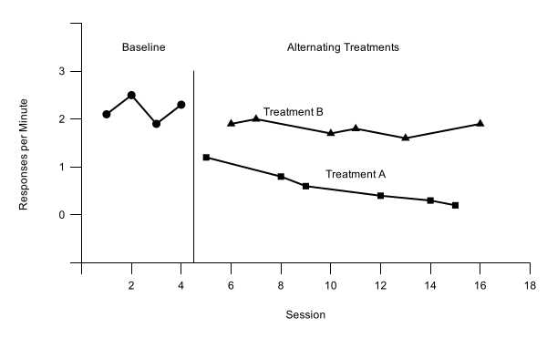
Practice data: practice-atd-data.xlsx, 16 sessions in A1:D17.
Give each condition its own column, just like a phase. During the alternating phase, each session's value goes in the column for the condition run that session. Each condition's column now has blank cells between its values.
| A | B | C | D | |
|---|---|---|---|---|
| 1 | Session | Baseline | Treatment A | Treatment B |
| 2–5 | 1–4 | 2.1 … 2.3 | ||
| 6 | 5 | 1.2 | ||
| 7 | 6 | 1.9 | ||
| 8 | 7 | 2.0 | ||
| 9 | 8 | 0.8 | ||
| 10 | 9 | 0.6 |
- Build the chart as usual. Select A1:D17, insert a line chart, and tick Use column A as labels, as in Lesson 2. Format it as in Lesson 3, with rate settings on the vertical axis: Min -1, Max 3, Major step 1, and format code 0;;0, so the labels are whole numbers. The practice rates peak at 2.5. Set the horizontal axis from 0 to 18, the first multiple of 2 past session 16, with a step of 2, and hide session 0 with the format code 0;;.
- Join each condition across its blank cells. A blank cell breaks a line, so each treatment would show as short pieces and lone points. In Customize›Chart style, tick Plot null values. The setting applies to every series in the chart. The Baseline path still stops at the phase change, because its column has no later values to join.
- Give each condition a different point shape. Google Sheets has no open (hollow) points, so use shapes. In Customize›Series, make every line black with 7px points (Apply to all series), then choose each treatment and set its Point shape and Point size: Treatment A Square, 8; Treatment B Triangle, 9. Baseline stays a 7px circle. Type 8 or 9 in the Point size box; squares and triangles look smaller than a circle of the same size.
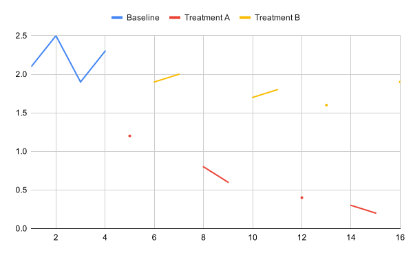
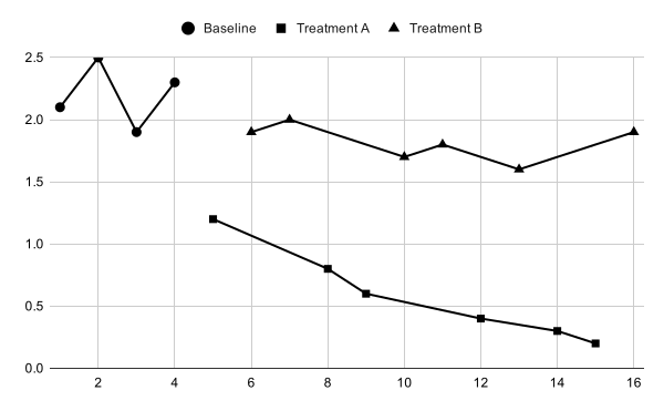
A path still breaks, or drops to zero? Look at the cell where it happens. A cell that only looks empty may hold a space or other text. Select it and press Delete to empty it.
- Add the phase-change line and the labels. Follow Lesson 4. The helper headings go in E1:G1 (Phase lines, Phase labels, Label text). Leave row 18 empty; the helper rows run from row 19 to row 24. The practice data change phase once, after session 4: 4.5 in A19:A20, with -1 and 3 in E19:E20. The label rows, 21 to 24, hold Baseline at 2.5 and Alternating Treatments at 10.5, both at 3.5, then the two treatment names. Set the data range to A1:G24, add Phase lines and Phase labels as series, and raise the vertical axis Max to 4 with the format code [>3]"";[<0]"";0, which hides the 4 label.
- Name the treatments beside their paths, not with a legend. A Google Sheets legend lists every series and can’t leave one out, so it would also list Phase lines and Phase labels. The last two label rows put the words Treatment A (at 11 and 0.85) and Treatment B (at 8.5 and 2.15) just above their own paths, as part of the Phase labels series. APA style allows labeling data paths directly instead of using a legend. For your own data, put each name close to its own path, where it covers no point or line of the other.
More than one phase change? Plot null values joins every series across its blank cells, the helper series included. The practice graph has a single phase-change line, so that changes nothing. If your own alternating treatments graph has a second phase change, such as a final best-treatment phase, check that the two phase-change lines stand apart. If they are joined, put the second line's two values in a column of its own and add that column as its own series.
Check your alternating treatments graph
- Treatment A and Treatment B are each one continuous path, joined across blank cells by Plot null values
- The Baseline path ends at session 4 and does not join either treatment
- Each condition has its own point shape: circles (Baseline), squares (Treatment A), triangles (Treatment B)
- One solid phase-change line at 4.5, from the horizontal axis to 3
- The labels Baseline and Alternating Treatments sit in the band at the top of the plot, centered over their phases
- Treatment A and Treatment B are labeled beside their own paths, and the graph has no legend
- Vertical axis −1 to 4 in steps of 1, with only 0 to 3 numbered
Then read the graph. Do the two treatment paths separate clearly, with little or no overlap, across the whole alternating phase? See what experimental control looks like in an alternating treatments design.
Multielement design (functional analysis)
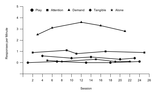
Practice data: practice-fa-data.xlsx, 25 sessions in A1:F26.
- One column per condition. Put session numbers in column A and one condition in each of columns B to F: Play, Attention, Demand, Tangible, and Alone. Type each session's rate under the condition run that session, so every row has exactly one rate. Type 0 for a session with no responding. Leave a cell blank only when that condition was not run in that session.
| A | B | C | D | E | F | |
|---|---|---|---|---|---|---|
| 1 | Session | Play | Attention | Demand | Tangible | Alone |
| 2 | 1 | 0 | ||||
| 3 | 2 | 0.9 | ||||
| 4 | 3 | 2.5 | ||||
| 5 | 4 | 0.6 | ||||
| 6 | 5 | 0.2 | ||||
| 7 | 6 | 3.1 | ||||
| 8 | 7 | 0.1 |
- Insert and format the chart. Select A1:F26, insert a line chart with Use column A as labels, and format it as in Lesson 3. On the vertical axis, set Min -1, Max 5, Major step 1, and format code 0;;0, so the labels are whole numbers. The practice rates peak at 3.6, so a maximum of 5 keeps the highest point well below the top of the plot. Set the horizontal axis from 0 to 26, one more than the last session, with a step of 2, and hide session 0 with 0;;.
- Join each condition across its blank cells. Tick Plot null values in Chart style, exactly as in step 2 of the alternating treatments design. Every condition's column has blanks between its values, so without this setting all five conditions show as lone dots.
- Use five shapes. Make every line black with 7px points, then give each test condition its own shape: Attention Square 8, Demand Triangle 9, Tangible Diamond 9, and Alone Star 10. Play, the control condition, stays a 7px circle. Sheets has no open points, so shape is the only way to tell the conditions apart in black and white. Whatever shapes you choose, keep them the same across all your figures.
- Skip the phase-change lines and phase labels. All five conditions alternate within one phase, so there is nothing to separate or name, and the graph needs no helper rows. The legend identifies the conditions instead.
- Turn the legend on. In Customize›Legend, set Position to Inside and Text color to black. The legend lists the conditions in column order, so the practice file puts the control condition, Play, first. To change the order, move the columns before you insert the chart. Whatever order you choose, use it in every figure.
Zero rates stay visible. With the floating zero from Lesson 3, sessions with no responding sit on the 0 line, just above the horizontal axis, instead of on it.
Check your multielement graph
- No phase-change lines, no phase labels, and no helper rows
- Five paths, each joined across blank cells by Plot null values
- Five point shapes that can be told apart in black and white
- A legend inside the plot, above the data, lists Play, Attention, Demand, Tangible, and Alone, in black text
- Sessions with no responding are typed as 0 and sit on the 0 line, above the horizontal axis
- Vertical axis −1 to 5 in steps of 1, with whole-number labels and the −1 label hidden
Then read the graph. Is responding in any test condition consistently higher than in the Play (control) condition, with little overlap? See Functional analysis: differentiated or not?
In the practice graph, Demand is clearly highest, at 2.5 to 3.6 responses per minute. Attention (0.8 to 1.1) and, at a lower level, Tangible (0.3 to 0.6) are also above Play (0 to 0.1) in all five cycles, with no overlap. Alone stays low (0.1 to 0.3) and overlaps Play at 0.1. Because each test condition is compared with Play, not just with the highest condition, this graph suggests escape plus attention, and possibly tangible: multiple control worth following up.
Changing criterion design
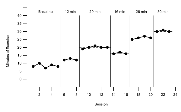
Practice data: practice-cc-data.xlsx, 23 sessions in A1:G24.
Why the subphases differ. The practice subphases last 3, 5, 3, 4, and 3 sessions, the criterion changes by different amounts (+8, −4, +10, and +4 minutes), and it steps back down from 20 to 16 minutes for a while. When behavior follows changes like these, time alone can’t explain them (see how the design shows control). The helper rows work the same for any subphase lengths and criteria: each criterion line spans exactly its own subphase.
- One column per subphase. Put Baseline, Phase 1, Phase 2, Phase 3, Phase 4, and Phase 5 in B1:G1, so the data path breaks at every criterion change. Select A1:G24, insert a line chart with Use column A as labels, and format it as in Lesson 3. On the vertical axis, set Min -5, Max 40, Major step 5, and format code 0;;0. The practice data peak at 31 minutes. Set the horizontal axis from 0 to 24, one more than the last session, with a step of 2, and hide session 0 with 0;;.
- Type the helper rows. Follow Lesson 4. The headings go in H1:K1: Phase lines, Phase labels, Label text, and Criterion. Leave row 25 empty. Rows 26 to 39 draw five phase-change lines at 5.5, 8.5, 13.5, 16.5, and 20.5, each from -5 to 40, with a separator row between lines. Rows 40 to 45 hold the labels Baseline, 12 min, 20 min, 16 min, 26 min, and 30 min at 3, 7, 11, 15, 18.5, and 22, all at 42.5. Rows 46 to 59 draw the criterion lines, shown below. Keep the phase-change lines solid.
- Make the criterion rows. Each criterion line is two rows. Column A runs from half a session before the subphase's first session to half a session after its last, and Criterion holds the criterion both times. For a criterion of 12 during sessions 6–8: 5.5 and 8.5 in column A, with 12 and 12 in column K. A separator row, with a position in column A and column K left empty, keeps one line from joining the next.
| A | K | ||
|---|---|---|---|
| 46 | 5.5 | 12 | ← 12 min, sessions 6–8 |
| 47 | 8.5 | 12 | |
| 48 | 8.5 | ← separator | |
| 49 | 8.5 | 20 | ← 20 min, sessions 9–13 |
| 50 | 13.5 | 20 | |
| 51 | 13.5 | ||
| 52 | 13.5 | 16 | ← 16 min, sessions 14–16 |
| 53 | 16.5 | 16 | |
| 54 | 16.5 | ||
| 55 | 16.5 | 26 | ← 26 min, sessions 17–20 |
| 56 | 20.5 | 26 | |
| 57 | 20.5 | ||
| 58 | 20.5 | 30 | ← 30 min, sessions 21–23 |
| 59 | 23.5 | 30 |
- Add the helper series. In the chart editor's Setup tab, set the Data range to A1:K59 and press Enter. Then use Add Series three times: Phase lines, Phase labels, and Criterion. Add the labels' words from Label text and format the lines and labels as in Lesson 4, Part B. Raise the vertical axis Max to 45, with the format code [>40]"";[<0]"";0.
- Make the criterion lines dashed. In Customize›Series, choose Criterion. Set Line color to black, Line dash type to the dashed line (third in the list), and Line thickness to 1px. Dashing keeps the criterion visibly different from the data path and the solid phase-change lines. All five criterion lines are one series, so this one setting dashes them all.
Changed a criterion? Edit its two cells in column K and its label in column J. The dashed line and the label move with the numbers.
Check your changing criterion graph
- The data path breaks at every phase change
- Five solid phase-change lines at 5.5, 8.5, 13.5, 16.5, and 20.5, from the horizontal axis to 40
- Five dashed criterion lines at 12, 20, 16, 26, and 30, each spanning only its own subphase
- Phase-change lines and criterion lines have no points
- The labels Baseline, 12 min, 20 min, 16 min, 26 min, and 30 min sit in the band at the top of the plot, centered over their subphases
- Vertical axis −5 to 45 in steps of 5, with only 0 to 40 numbered
Then read the graph. Does responding shift to each new criterion soon after it changes and stay near it until the next change? See what experimental control looks like in a changing criterion design.