

Overview › Build it in Google Sheets › Lesson 2
Create the chart
Insert a line chart, tell Google Sheets to use the session numbers in column A as its horizontal axis, check that it read your columns correctly, and move it off your data.
You will be able to
- Insert a line chart that uses the session numbers in column A as a number line on its horizontal axis, and fix one that doesn’t.
- Explain why a single-case graph in Google Sheets uses a line chart, not a scatter chart.
- Move the chart off your data and keep it at Sheets’ default size.
Why a line chart and not a scatter chart? The Excel lessons use a scatter chart, because Excel's line chart spaces the sessions evenly as text. In Google Sheets it is the other way around. Sheets' scatter chart can't draw a data path: its series settings have point size and shape, but no option to join the points with a line. Sheets' line chart joins them, and once it uses column A as a number line (step 4), it places every point at its real session number. That lets you put a phase-change line exactly at session 5.5 in Lesson 4.That keeps each condition's points at the sessions when they actually ran.
Steps
- Select the data, including the headings. Click cell A1 and drag across to the last phase columnParticipant 1's last phase columnthe last condition column and down to the last row of data (E21 in practice-reversal-data.xlsx), so the selection is A1:E21. You can also click A1 and then Shift-click E21. That last cell is empty, because the final session in the practice data wasn't an Alone session. Include it anyway, so the selection covers every session. That selects only the Session column and Participant 1's two columns. The practice file also holds Participants 2 and 3 in the columns to the right. Leave them out for now: this lesson and the next two build Participant 1's tier as a full-size chart, and Lesson 5 adds the other tiers.
- Insert a chart. Choose Insert›Chart. Sheets adds a chart and opens the chart editor on the right, on its Setup tab. It guesses a Column chart and treats Session as one of the series. The next two steps fix both. If a suggestion such as Convert to table or Analyze this data pops up next to your data, close it with its X.
- Change the chart type to a line chart. In the chart editor's Setup tab, open the Chart type list and choose Line chart, the first icon in the Line group.
- Use column A as the horizontal axis. Near the bottom of the Setup tab, tick Use column A as labels. Leave Treat labels as text unticked: then the session numbers become a number line on the horizontal axis (2, 4, 6 …), not a row of evenly spaced labels. You don't need to tick Use row 1 as headers; the series still take their names from the headings in row 1.
- Compare your chart with this picture. You should see four colored lines, one per phase, with a gap at each phase change. There is no chart title, but there are gridlines and a legend at the top. Lesson 3 removes them. You should see three colors, one for each condition column. The Baseline points are joined into one path, but Treatment A and Treatment B show only short pieces of line, where the same treatment ran in back-to-back sessions. A point with no neighbor to join shows as a tiny dot or not at all. You should see almost nothing but tiny dots in five colors. In the practice data no condition ran in back-to-back sessions, so no two points of a condition are joined. That is expected for now. Each condition's column has a blank cell for every session in which a different condition ran, and a blank cell breaks the line. Lesson 3 connects each condition's points across those blanks. There are also gridlines and a legend at the top, which Lesson 3 removes. The lines have no points yet: a new line chart starts with its Point size set to None. Lesson 3 adds them.
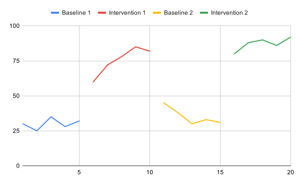
Doesn't match? If one of the lines is named Session, or the horizontal axis shows evenly spaced labels instead of a number line, check step 4: Use column A as labels must be ticked and Treat labels as text unticked. If the chart still has bars, redo step 3. If some session numbers in column A sit at the left of their cells, they are stored as text; retype them as plain numbers (Lesson 1, step 6). If nothing helps, delete the chart (click it, then its three-dot menu › Delete chart), check that A1 contains the word Session, select the data again, and insert a new chart.
- Move the chart off your data. Close the chart editor with the X at its top right. Point at the chart's edge, then drag the chart to an empty spot, so it covers none of your cells. Lesson 4 types helper rows under your data, using column A and columns F, G, and H, so keep the chart off those columns and off the rows under your data. Keep it off columns D to G, which hold Participants 2 and 3, and off columns H, I, and J and the rows under your data, where Lesson 4 types helper rows. Lesson 5 also uses columns K and L. Your graph needs no helper rows, so anywhere clear of your data will do. A chart floats over the sheet, so you can move it again at any time.
- Keep the default size. Google Sheets has no box for typing a chart's size; you change it by dragging the handles on the chart's edges. A new chart is 600 × 371 pixels. Keep that size: the pictures in these lessons were made at it, and in Lesson 7 the chart downloads at the size it has on the sheet. Lesson 5 makes each tier shorter by dragging, once Participant 1's tier is finished.
Why not resize it? Sheets draws the chart's text at fixed sizes, so a bigger or smaller chart changes how large the text looks next to the plot. At the default size, your chart matches the pictures here. In Lesson 7 you check that the text is still between 8 and 14 points, as APA asks, at the size the figure is printed.
The most common mistake
Putting every value in one column and charting that column. The line then climbs straight from the last baseline point into intervention, so the phase change disappears into one continuous line. When conditions alternate, the result is worse: one zigzag line runs through every condition in session order, so no one can tell which point belongs to which condition. If your chart shows a single line, go back to Lesson 1: Set up your data and give each phasecondition its own column.