

Overview › Build it in Google Sheets › Lesson 5
Multiple baseline graphs
A multiple baseline figure is a stack of identical graphs, one per participant, behavior, or setting. They share one horizontal axis and are joined by a stepped phase-change line. You built the top tier in Lessons 1 to 4. Here you make it short, copy it, and point each copy at its own data in Google Sheets. Sheets can’t combine charts into one figure, so you then stack the three tiers in Google Slides.
You will be able to
- Make a short tier, copy it for each participant, and point each copy at its own data and its own phase-change line.
- Stack the tiers in Google Slides so their plots line up, with phase labels on the top tier only, one vertical axis title, and session numbers on the bottom tier only.
- Add the tier names and draw the stepped line that joins the phase changes across tiers.
Not needed for your graph. This lesson is only for multiple baseline graphs, and your graph type is set to Reversal (ABAB). Your graph is complete after Lesson 4, so go on to Lesson 7: Download and place the figure.Go on to Lesson 6: Alternating treatments, multielement, and changing criterion. To build a multiple baseline graph instead, switch to Multiple baseline.
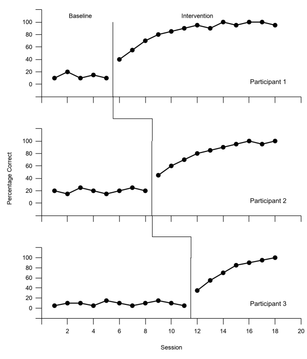
Practice data: practice-multiple-baseline-data.xlsx. It holds all three tiers. Lessons 1 to 4 used Participant 1 in columns A:C. This lesson adds the other two.
Part A: Check the data layout
The practice data use one Session column and two columns per tier, one for Baseline and one for Intervention. This is Lesson 1's rule applied to each tier. Participant 1 is in columns B and C, Participant 2 in D and E, and Participant 3 in F and G. Lesson 4's helper columns, H to J, sit to the right of them, and this lesson adds two more, K and L.
| A | B | C | D | E | F | G | |
|---|---|---|---|---|---|---|---|
| 1 | Session | P1 Baseline | P1 Intervention | P2 Baseline | P2 Intervention | P3 Baseline | P3 Intervention |
| 2 | 1 | 10 | 20 | 5 | |||
| 3 | 2 | 20 | 15 | 10 | |||
| 4 | 3 | 10 | 25 | 10 | |||
| 5 | 4 | 15 | 20 | 5 | |||
| 6 | 5 | 10 | 15 | 15 | |||
| 7 | 6 | 40 | 20 | 10 | |||
| 8 | 7 | 55 | 25 | 5 | |||
| 9 | 8 | 70 | 20 | 10 | |||
| 10 | 9 | 80 | 45 | 15 | |||
| 11 | 10 | 85 | 60 | 10 | |||
| 12 | 11 | 90 | 70 | 5 | |||
| 13 | 12 | 95 | 80 | 35 | |||
| 14 | 13 | 90 | 85 | 55 | |||
| 15 | 14 | 100 | 90 | 70 | |||
| 16 | 15 | 95 | 95 | 85 | |||
| 17 | 16 | 100 | 100 | 90 | |||
| 18 | 17 | 100 | 95 | 95 | |||
| 19 | 18 | 95 | 100 | 100 |
Part B: Make the top tier short
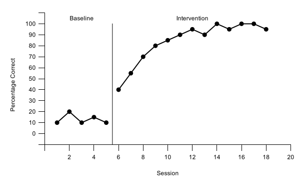
- Start from your tier 1 chart. Lessons 1 to 4, with Multiple baseline chosen in the Graph box, built Participant 1 (columns A:C) as a finished chart: black axes, a floating zero, axis titles, a phase-change line after session 5, and the labels Baseline and Intervention. Every tier will be a copy of this chart, so fix anything in it now. If you haven't built it yet, start at Lesson 1.
- Make it short. Click the chart. Sheets has no boxes for a chart's size, so drag the handle in the middle of its bottom edge up until the chart is about 230 pixels tall, a little under two-thirds of its first height (600 × 233): about 11 rows at the default row height. The exact height matters less than the copies all matching, and copies keep the size of the chart you copy.
- Rescale the vertical axis for a short tier. A short tier has no room for a number every 10. Open the chart editor (the chart's three-dot menu › Edit chart) and click Customize. In Vertical axis, set Min to -20 and Max to 120. In Gridlines and ticks, choose Vertical axis and set Major step to 20. The format code from Lesson 4, [>100]"";[<0]"";0, still hides the −20 and 120 labels, so zero floats one step above the horizontal axis and the band from 100 to 120 holds the phase labels.
- Update tier 1's helper rows to match. Change the bottom of the phase-change line, cell H21, from -10 to -20, so the line still reaches the horizontal axis. Change the label heights, I23:I24, from 105 to 110, the middle of the new band.
- Hide the session numbers on this tier. In Horizontal axis, open Number format, choose Other custom formats, type ;;; (three semicolons), and click Apply. The numbers disappear; the axis line and tick marks stay. Then open Chart & axis titles, choose Horizontal axis title, and delete its text.
- Blank the vertical axis title, but keep it. Still in Chart & axis titles, choose Vertical axis title and replace Percentage Correct with a single space. The tier then keeps the same left margin as the middle tier, which will carry the real title, so the three vertical axes line up.
Part C: Copy the tier and point each copy at its own data
Each tier gets its own phase-change line, from its own two helper rows. Tier 1 already uses rows 21 and 22 (column H). Tiers 2 and 3 get two rows each under the label rows, each in a column of its own, so each chart can take in its own line and no other.
| A | H | I | J | K | L | |
|---|---|---|---|---|---|---|
| 1 | Session | Phase lines | Phase labels | Label text | Tier 2 line | Tier 3 line |
| 21 | 5.5 | -20 | ||||
| 22 | 5.5 | 100 | ||||
| 23 | 3 | 110 | Baseline | |||
| 24 | 12 | 110 | Intervention | |||
| 25 | 8.5 | -20 | ||||
| 26 | 8.5 | 100 | ||||
| 27 | 11.5 | -20 | ||||
| 28 | 11.5 | 100 |
- Type the tier 2 and tier 3 rows. Type Tier 2 line in K1 and Tier 3 line in L1. Then type 8.5 in A25:A26 with -20 and 100 in K25:K26, and 11.5 in A27:A28 with -20 and 100 in L27:L28. Tier 1's data range grows to A1:C28,H1:J28 by itself. That is fine: its columns are empty in the new rows.
- Copy the chart twice. Click the chart, then its three-dot menu, and choose Copy chart. Click an empty cell below the chart, such as B30, and paste with Ctrl+V (⌘+V on a Mac). Click a cell farther down, such as B48, and paste again. You now have three identical charts.
- Point tier 2 at its own data. Click the copy you pasted at B30 and open the chart editor on its Setup tab. Click the Data range box, replace what is there with A1:A28,D1:E28,K1:K28, and press Enter. The series all disappear (Add a series to start), and a Combine ranges setting appears, set to Horizontally; keep it. Click Add Series three times and choose, in this order, P2 Baseline, P2 Intervention, and Tier 2 line. The copy keeps its formatting by position, so the two data series come in black with 7px points and the line thin and black, as on tier 1.
- Type the real vertical axis title on tier 2. Tier 2 is the middle tier. In Customize›Chart & axis titles, choose Vertical axis title and replace the space with Percentage Correct, so one title serves the whole figure and sits near its middle.
- Set up tier 3 the same way.
Click the copy at B48. Set its Data range to A1:A28,F1:G28,L1:L28, and add P3 Baseline, P3 Intervention, and Tier 3 line, in that order. Leave its vertical title a single space. Then give it back what only the bottom tier shows:
- the session numbers: in Horizontal axis, open Number format, choose Other custom formats, type 0;;, and click Apply. The numbers return, and session 0 stays hidden, as in Lesson 3
- the horizontal axis title: in Chart & axis titles, choose Horizontal axis title and type Session
Tier 3's plot is a little shorter. All three charts are the same height, but tier 3's also has to hold the session numbers and the Session title, so its plot comes out a little shorter than the others. You can see this in the finished figure above. If you want every tier to show exactly the same vertical scale, drag tier 3's bottom handle down a little before you go on, until its plot is as tall as tier 2's, and make the slide a little taller in Part D to fit it.
Part D: Stack the tiers in Google Slides
Google Sheets can’t combine charts into one figure, so you stack them on a slide in Google Slides, with each tier linked to its chart in your spreadsheet.
- Open a blank presentation. In your web browser, go to slides.new, or open Google Slides and start a blank presentation. Delete the title and subtitle boxes: click the slide, press Ctrl+A (⌘+A on a Mac), then press Delete.
- Make the slide the size of the figure. Choose File›Page setup, choose Custom, type 6.5 by 7.6 inches, and click Apply. A width of 6.5 inches fills a page with 1-inch margins.
- Bring in the three tiers. Choose Insert›Chart›From Sheets. Pick your spreadsheet and click Insert at the bottom right. The next list shows every chart in the file; pick tier 1. Leave Link to spreadsheet ticked and click Import. Do the same for tier 2 and tier 3.
- Size each tier and put it in place. Select a chart and click Format options in the toolbar. Under Size & Rotation, tick Lock aspect ratio and set Width to 6.5 in; the height becomes 2.52. Under Position, set X to 0 and Y to 0 for tier 1, 2.52 for tier 2, and 5.04 for tier 3. Because the three charts have the same size and the same axis margins, their vertical axes now form one straight column. If Height doesn’t read 2.52 (your tier is a little taller or shorter), use your height h instead: Y = 0, h, and 2h; a slide 3h tall; and the tier names moved by the same amounts. If one chart is hidden behind another, click a chart you can see and press Tab: the selection moves to the next object on the slide.
Part E: Add the tier names and the stepped line
- Add the tier names. Choose Insert›Text box, drag a small box, and type Participant 1. Select the text and set the font size to 10 (Arial is already the font) and the text color to black. Press Esc so the box itself is selected, not its text, then press Ctrl+D (⌘+D on a Mac) to duplicate it, and change the copy to Participant 2; do it again for Participant 3. Then select each box, open Format options › Position, and set X to 5.2 and Y to 1.55, 4.07, and 6.25, which puts each name inside its tier's plot, at the bottom right.
- Draw the step from tier 1 to tier 2. Choose Insert›Line›Polyline. Click on tier 1's phase-change line where it meets the horizontal axis. Click straight below that point, in the gap between the tiers. Click straight above tier 2's phase-change line, at the same height. Then double-click on the top of tier 2's line to finish.
- Draw the step from tier 2 to tier 3. Do the same from the bottom of tier 2's line to the top of tier 3's.
- Format both steps. Click one step, hold Shift, and click the other. Set the Border color (the line color) to black and the Line weight to 1px, the same as the phase-change lines.
Lesson 7 downloads the slide as a picture file and puts it in your manuscript.
The tiers stay linked to your data. Each chart on the slide is linked to its chart in the spreadsheet. When you change the data in Google Sheets, the chart in Slides offers an Update button; click it to bring in the change. The tier names and the stepped line are drawn on the slide, so check that they still line up after a change to the phase timing.
Across participants, behaviors, or settings? The figure is built the same way. Only the tier names change (for example, Home, School, Clinic). More than three tiers? Copy a middle tier again, give it its own two helper rows and its own helper column, make the slide taller, and move the real vertical title to the tier nearest the middle.
Check before moving on
- Every tier has the same axes: horizontal 0 to 20, vertical −20 to 120 in steps of 20, with only 0 to 100 numbered, so zero floats above the horizontal axis
- Each tier plots its own Baseline and Intervention columns, and its own phase-change line, at 5.5, 8.5, and 11.5, from the horizontal axis to 100
- Phase labels appear on the top tier only, in the band above its data
- One vertical axis title, on the middle tier; the other two keep a single space
- Session numbers (with 0 hidden) and the Session title on the bottom tier only
- On the 6.5 × 7.6 in slide, each tier is 6.5 in wide and the three vertical axes form one straight column
- Each tier is named inside its plot, in Arial 10 pt, black
- Two black 1px stepped lines meet each tier's phase-change line with no gaps