

Overview › Visual analysis › Lesson 4
Visual aids and the dual-criteria method
Lines drawn from baseline data can make judgments more consistent. The conservative dual-criteria method turns them into a clear decision rule.
You will be able to
- Apply the conservative dual-criteria method to an AB comparison and decide whether it meets the criterion.
- Build the shifted mean and trend lines in Excel from baseline data.
- Explain why meeting the criterion is one demonstration of an effect, not experimental control.
Common visual aids
- Mean or median lines summarize the level of each phase (see level).
- Trend lines, such as a least-squares line or a split-middle line, summarize direction and steepness. Extending the baseline trend into the next phase shows what baseline predicted.
- Stability bands draw an envelope around the median to judge whether a phase is stable enough to change. A common rule calls a phase stable when about 80% of its points fall within ±25% of its median (Lane & Gast, 2014). Lesson 6 works through one.
Working graphs, not publication graphs. Aids help you make decisions while a study runs. Leave them off publication figures unless your analysis depends on them, and say so in the figure note.
The conservative dual-criteria (CDC) method
Fisher, Kelley, and Lomas (2003) developed a structured rule for AB comparisons. It improved how accurately people judged graphs, and later studies taught it to students quickly (Stewart et al., 2007).
- Draw the baseline mean line and extend it through the intervention phase.
- Draw the baseline trend line (least squares) and extend it through the intervention phase.
- Shift both lines by 0.25 of the baseline standard deviation in the direction you expect behavior to change, down for a decrease or up for an increase. This shift is what makes the method conservative.
- Count the intervention points that fall beyond both lines in the expected direction.
- Compare the count with the number needed for the number of intervention points (table below). If the count reaches it, this AB comparison shows a systematic change: more points fell beyond both lines than chance variation would be likely to produce.
| Intervention points | Points needed beyond both lines |
|---|---|
| 5 | 5 |
| 6–7 | 6 |
| 8 | 7 |
| 9–10 | 8 |
| 11–12 | 9 |
| 13 | 10 |
| 14 | 11 |
| 15–17 | 12 |
| 18–19 | 13 |
| 20–21 | 14 |
| 22–23 | 15 |
These are the criteria Fisher et al. (2003, p. 399) published, as reprinted by Swoboda et al. (2010, Table 1). They are based on a binomial test that gives each intervention point a .5 chance of falling beyond both lines, and they assume you predicted the direction of change before looking at the data. The table covers 5 to 23 intervention points.
One comparison is one demonstration. Meeting the criterion shows a systematic change in a single AB comparison. It doesn't show that the intervention caused the change, and it isn't experimental control. To use the method with a reversal or multiple baseline design, apply it to each phase change or each tier separately. Draw the lines from the phase just before the change, and expect the change in the direction that phase change should produce: back toward baseline when the intervention is withdrawn. Control still needs at least three demonstrations. This extension comes from Swoboda et al. (2010), who describe it as an informal generalization that still needs formal evaluation. Lesson 5 works through it, and has you calculate the lines yourself.
Adding the lines in Excel
Don't use Excel's built-in trendline for this method. It draws an unshifted least-squares line, and it can't be moved 0.25 SD: Set Intercept refits the line rather than shifting it. Instead, build both lines as two-point helper series, the same way you built phase-change lines in Excel Lesson 4.
The example uses the AB practice file, practice-ab-data.xlsx. Sessions are in A2:A16, baseline data in B2:B6 (sessions 1–5), and intervention data in C7:C16 (sessions 6–15). The goal is to decrease problem behavior, so both lines shift down.
| L | M | N | O | P | Q | |
|---|---|---|---|---|---|---|
| 1 | Baseline | Value | X | Mean line | Trend line | |
| 2 | Mean | 57.80 | 1 | 56.08 | 54.08 | |
| 3 | SD | 6.87 | 15 | 56.08 | 68.08 | |
| 4 | Shift | -1.72 | ||||
| 5 | Slope | 1.00 | ||||
| 6 | Intercept | 54.80 |
- Calculate the baseline statistics.
In L1 and M1 type Baseline and Value, and in L2:L6 type the labels shown above. Then type these formulas in M2 to M6:
- M2, mean:
=AVERAGE($B$2:$B$6) - M3, standard deviation:
=STDEV.S($B$2:$B$6) - M4, shift:
=-0.25*M3(for an expected increase, use=0.25*M3) - M5, slope:
=SLOPE($B$2:$B$6,$A$2:$A$6) - M6, intercept:
=INTERCEPT($B$2:$B$6,$A$2:$A$6)
- M2, mean:
- Build the line table.
In O1:Q1 type X, Mean line, and Trend line. In O2 type 1, the first baseline session, and in O3 type 15, the last intervention session. In P2 type
=$M$2+$M$4and in Q2 type=$M$6+$M$5*O2+$M$4, then fill both down to row 3. Both lines are straight, so two points are enough to draw each one. - Add the two lines. Click the chart and open Chart Design›Select Data. Add a series (Add on Windows, + on Mac) named Mean line. Click in X values, delete anything in it, and drag across O2:O3. Click in Y values, delete the placeholder, and drag across P2:P3. Add a second series named Trend line the same way, with X values O2:O3 and Y values Q2:Q3. Click OK to close Select Data.
- Format the lines. Double-click each line to open Format Data Series. Under Fill & Line › Line, choose Solid line and a thin width, and give the two lines different dash types so you can tell them apart in black and white. Under Marker › Marker Options, choose None.
- Count and compare.
Count the intervention points below both lines (above both for an expected increase), and compare the count with the table above. To check your count,
=SUMPRODUCT((C7:C16<$M$2+$M$4)*(C7:C16<$M$6+$M$5*A7:A16+$M$4))returns the number of intervention points below both lines. For an expected increase, change both<signs to>.
Result for the practice data. The baseline mean is 57.8 and the standard deviation is about 6.87, so the shift is about −1.72. The baseline slope is 1.00 and the intercept is 54.8. The shifted mean line sits at about 56.1, and the shifted trend line runs from about 54.1 at session 1 to 68.1 at session 15. All 10 intervention points fall below both lines. With 10 intervention points, 8 are needed, so this comparison meets the criterion. It is still one AB comparison: a systematic change, not experimental control.
Other aids. An unshifted mean line for any phase is the same kind of two-point series, with both Y values set to =AVERAGE(...) of that phase and X values at the phase's first and last sessions. For a quick look at the baseline trend, select the baseline series and add a linear trendline (Chart Elements › Trendline on Windows, Chart Design › Add Chart Element › Trendline on Mac), then set Forecast Forward to the number of intervention sessions. Count dual-criteria points against the two helper lines, never against this trendline.
Practice
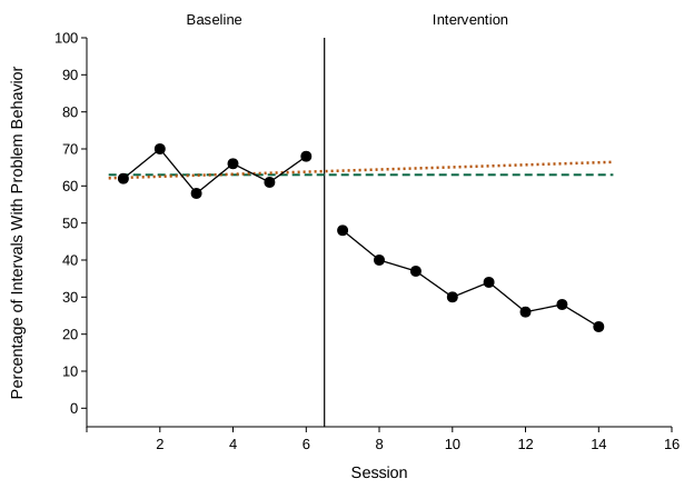
Every practice graph is a single AB comparison. The dashed line is the shifted mean and the dotted line is the shifted trend. Both come from baseline and are already shifted 0.25 SD toward the expected change. Count the intervention points beyond both lines. When your count is right, decide whether the graph meets the criterion; the question lists the points needed, as in the table above. An item counts only when both answers are right.