
Overview › Visual analysis › Lesson 6
Variability and stability in depth
Lesson 1 described variability by the range. Here you measure it from every data point: each point's distance from the level line, the sum of squares, the variance, and the standard deviation. Then you compare variability within and across phases, judge whether a phase is stable, and see what a trend does to it.
You will be able to
- Find each data point's distance from its phase's level line, and explain why the distances always add to zero.
- Calculate a phase's sum of squares, variance, and standard deviation, by hand and in Excel.
- Compare variability across phases, each measured around its own level line.
- Judge whether a phase is stable with a stability envelope, and measure variability around a trend line when the data trend.
- Work through new graphs step by step, reaching 8 of your last 10 in the practice.
Why the range isn't enough
The range uses only the two most extreme points. One unusual session can make a steady phase look variable, and two phases with the same range can bounce around their level very differently. Measuring every point's distance from the level line uses all the data, so each session counts.
Distance from the level line
Draw the phase's level line at its mean. Each point's distance from that line is its value minus the mean: positive for a point above the line, negative for a point below it, and 0 for a point on it.
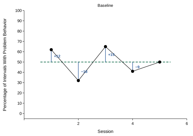
Add the distances and you get 0: 12 − 18 + 15 − 9 + 0 = 0. You always will. The mean is the balance point of the data, so the distances above it cancel the distances below it. To measure how far the points spread, the signs have to go. There are two ways:
- Mean absolute deviation. Average the distances without their signs: (12 + 18 + 15 + 9 + 0) ÷ 5 = 10.8. A typical session is about 11 points from the level line. Excel's
=AVEDEVreturns it. - Variance and standard deviation. Square the distances, so larger distances count for more. This is the measure behind the shift in the dual-criteria method and behind most statistics, so it is worth calculating by hand once.
Variance and standard deviation by hand
| Session | Value | Distance from the level (value − 50) | Squared distance |
|---|---|---|---|
| 1 | 62 | +12 | 144 |
| 2 | 32 | −18 | 324 |
| 3 | 65 | +15 | 225 |
| 4 | 41 | −9 | 81 |
| 5 | 50 | 0 | 0 |
| Total | 250 | 0 | 774 |
- Level. 250 ÷ 5 = 50.
- Distances. Subtract the level from each value.
- Sum of squares. Square each distance and add the squares: 144 + 324 + 225 + 81 + 0 = 774.
- Variance. Divide the sum of squares by n − 1, one less than the number of points: 774 ÷ 4 = 193.5. Its units are squared, percentage points squared here, so it is hard to picture on its own.
- Standard deviation. Take the square root of the variance: √193.5 = 13.9. It is back in the units of the data: a typical session is about 14 percentage points from the level line.
Why n − 1? The level line comes from the same five points, so the points sit a little closer to it than they would to the behavior's true level. Dividing by n − 1 instead of n makes up for that. Excel's VAR.S and STDEV.S divide by n − 1, and VAR.P and STDEV.P divide by n. Use the .S versions, as the dual-criteria lessons do.
In Excel
With the sessions in A2:A6 and the values in B2:B6:
- Level:
=AVERAGE(B2:B6)in B7 - Each distance:
=B2-$B$7in C2, filled down to C6 - Each squared distance:
=C2^2in D2, filled down to D6, and the sum of squares,=SUM(D2:D6) - The same sum of squares in one step:
=DEVSQ(B2:B6) - Variance and standard deviation:
=VAR.S(B2:B6)and=STDEV.S(B2:B6)
Build the distance and squared-distance columns at least once. They show where each number comes from, and which sessions add the most to the variance: here session 2, whose squared distance, 324, is over 40% of the total.
Within a phase and across phases
Variability within a phase is the bounce from session to session around that phase's own level. To compare phases, find each phase's variance around its own level line, then compare the standard deviations, which are in the units of the data.
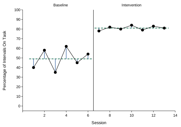
- Use one level line per phase. Around one line across all 13 sessions, at 66.2, the variance would be about 325, far more than either phase's, because the jump in level between phases would count as bounce.
- A change in variability is part of what changed. When variability drops, behavior became more predictable. When it rises, the new level is harder to pin down, and the phase may need more sessions before you can judge it. Report it alongside the change in level.
- Compare similar phases too. Two baseline phases at the same level but with very different standard deviations aren't fully alike, which weakens consistency.
Stability before a phase change
Change phases when the data are steady enough to predict what would happen next. A stability envelope turns that into a rule: draw the phase's median, then lines 25% of the median above and below it. A common rule calls the phase stable when about 80% of its points fall inside the envelope (Lane & Gast, 2014).
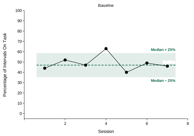
- Median. Sort the points and take the middle one: 40, 44, 46, 47, 49, 52, 63. Excel:
=MEDIAN(B2:B8). - Envelope. The lower edge is 0.75 × the median and the upper edge 1.25 × the median.
- Count. Count the points between the edges. Excel:
=COUNTIFS(B2:B8,">="&E2,B2:B8,"<="&E3), with the lower edge in E2 and the upper edge in E3. - Decide. Compare the count with 80% of the number of points, rounded up.
Read the envelope with the graph. The envelope is a percentage of the median, so it is narrow when the median is low: around a median of 8, it reaches only 2 either way. And it judges spread, not trend: data that rise steadily can stay inside a wide envelope. Check the trend separately before you change phases.
When the data trend
A level line is flat. When a phase trends, each point's distance from the level line includes the trend itself, so the variance overstates the bounce. Measure from the trend line instead, using its value at each session (intercept + slope × session, as in Lesson 5).
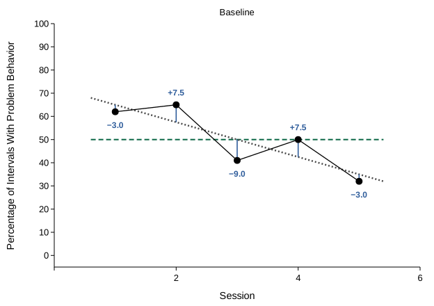
The variance ignores order: the same five values have the same variance in any order. The graph doesn't. That is why visual analysis describes trend and variability separately: first the trend, then how far the points scatter around it. (To turn the scatter around a trend line into a variance, statisticians divide its sum of squares by n − 2, because the line uses two values from the data, its slope and its intercept.)
Practice
Each graph works in steps. Most ask you to calculate a phase's level, distances, sum of squares, variance, and standard deviation by hand. Others compare two phases, test stability with an envelope, or measure the bounce around a trend line. The data table is open, with the exact values. Round as each step asks; answers within a rounding step are accepted. After a wrong step, the right answer appears so you can carry on, and a graph counts toward mastery only when every step is right.