

Overview › Visual analysis › Lesson 5
Applying the dual-criteria method
Lesson 4 drew the lines for you. Here you calculate them from the data, find the line that decides each count, and apply the method to every phase change of a reversal design and every tier of a multiple baseline design.
You will be able to
- Calculate the baseline mean, standard deviation, shift, slope, and intercept, and the value of each shifted line at any session.
- Tell which line is stricter during intervention, and explain how a baseline trend decides it.
- Apply the method to each phase change of a reversal design and each tier of a multiple baseline design, and count the demonstrations of an effect.
- Work through new graphs step by step, reaching 8 of your last 10 in the practice.
Build the lines from the data
The worked example is an AB graph of problem behavior, so the goal is a decrease. Baseline has five sessions. Work along with a calculator or a spreadsheet. In the table, x is the session, y is the value, and x̄ and ȳ are their means: 3 and 61.
| Session (x) | Value (y) | x − x̄ | y − ȳ | (y − ȳ)² | (x − x̄)(y − ȳ) |
|---|---|---|---|---|---|
| 1 | 64 | −2 | 3 | 9 | −6 |
| 2 | 66 | −1 | 5 | 25 | −5 |
| 3 | 58 | 0 | −3 | 9 | 0 |
| 4 | 62 | 1 | 1 | 1 | 1 |
| 5 | 55 | 2 | −6 | 36 | −12 |
| Total | 305 | 0 | 0 | 80 | −22 |
- Mean. 305 ÷ 5 = 61.0.
- Standard deviation. The squared distances from the mean add to 80. Divide by n − 1 = 4 for the variance, 20, and take the square root: the standard deviation is 4.47. This is what
=STDEV.Sreturns. Lesson 6 explains each part of this calculation. - Shift. 0.25 × 4.47 = 1.12. The goal is a decrease, so both lines move down: the shift is −1.12.
- Shifted mean line. 61.0 − 1.12 = 59.88, about 59.9. The line is flat, so it has this value at every session.
- Slope and intercept. The slope is the last column's total divided by the total of (x − x̄)², which is 4 + 1 + 0 + 1 + 4 = 10: −22 ÷ 10 = −2.2 points per session. The intercept is ȳ − slope × x̄ = 61 − (−2.2 × 3) = 67.6. Excel's
=SLOPEand=INTERCEPTreturn the same values. - Shifted trend line. At any session, its value is intercept + slope × session + shift. At session 6: 67.6 − 2.2 × 6 − 1.12 = 53.28. At session 15: 67.6 − 2.2 × 15 − 1.12 = 33.48. Always use the session number itself, not the point's place in the intervention phase.
- Find the stricter line. For a decrease, a point counts only if it falls below both lines, so at each session the lower line decides. The two lines cross at the middle of baseline, session 3. Baseline was already falling, so after that the trend line stays below the mean line: at session 6 it is 53.3, against 59.9. The trend line decides every intervention point.
- Count and compare. Count the intervention points below both lines and compare the count with the table in Lesson 4.
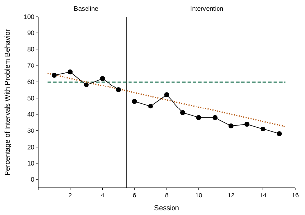
| Session | Value | Shifted mean | Shifted trend | Below both? |
|---|---|---|---|---|
| 6 | 48 | 59.9 | 53.3 | Yes |
| 7 | 45 | 59.9 | 51.1 | Yes |
| 8 | 52 | 59.9 | 48.9 | No, above the trend line |
| 9 | 41 | 59.9 | 46.7 | Yes |
| 10 | 38 | 59.9 | 44.5 | Yes |
| 11 | 38 | 59.9 | 42.3 | Yes |
| 12 | 33 | 59.9 | 40.1 | Yes |
| 13 | 34 | 59.9 | 37.9 | Yes |
| 14 | 31 | 59.9 | 35.7 | Yes |
| 15 | 28 | 59.9 | 33.5 | Yes |
Why the trend line mattered here. Baseline was already falling about 2 points per session. Judged against the mean line alone, all 10 intervention points would count. The trend line asks the harder question: did behavior fall further than the baseline trend predicted? When baseline trends away from the goal instead, the mean line is the stricter one, and the trend line adds nothing to the count.
Every phase change of a reversal design
A reversal (ABAB) design has three phase changes, and each one is its own AB comparison (Swoboda et al., 2010). Test each one in turn:
- Draw both lines from the phase before the change. Use that phase's values for the mean and standard deviation, and its own session numbers for the slope and intercept.
- Shift them toward the change you expect at that phase change. When the intervention starts, that is toward the goal. When it is withdrawn, it is back toward baseline, the opposite way.
- Count and compare. Count the points in the phase after the change that fall beyond both lines in that direction, and compare the count with the table for that phase's number of points.
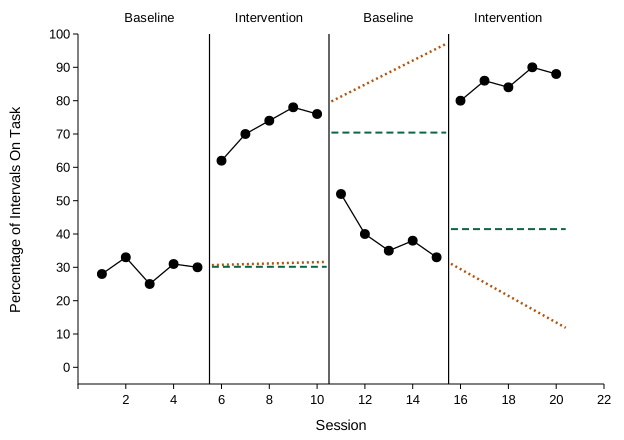
| Phase change | Lines from | Shift | Shifted mean | Shifted trend | Beyond both lines | Result |
|---|---|---|---|---|---|---|
| Baseline 1 to Intervention 1 | Baseline 1, sessions 1–5 | Up, +0.76 | 30.2 | 30.8 to 31.6 | 5 of 5 above | Meets |
| Intervention 1 to Baseline 2 | Intervention 1, sessions 6–10 | Down, −1.58 | 70.4 | 81.2 to 95.6 | 5 of 5 below | Meets |
| Baseline 2 to Intervention 2 | Baseline 2, sessions 11–15 | Up, +1.86 | 41.5 | 29.5 to 13.5 | 5 of 5 above | Meets |
Each tested phase has 5 points, so all 5 must fall beyond both lines: with 5 points, 5 are needed. All three phase changes meet the criterion, which gives three demonstrations of an effect at three points in time, the number experimental control needs. Notice the second and third tests. Intervention 1 was rising, so its trend line climbs steeply through Baseline 2, and the mean line decides there. Baseline 2 was falling, so in Intervention 2 the mean line decides again.
Short phases need every point. With 5 or 6 points in a phase, every point must fall beyond both lines, so one point in the wrong place means that phase change doesn't meet the criterion, even when the graph looks convincing. Longer phases leave a little room: 7 points need 6, and 10 need 8.
Every tier of a multiple baseline design
In a multiple baseline design, each tier is its own AB comparison. Draw each tier's lines from that tier's own baseline, extend them through its intervention phase, and count that tier's intervention points. Three tiers that each meet the criterion give three demonstrations, at three different times.
Also read the tiers together. When one tier starts intervention, the tiers still in baseline should stay where they were. The method tests each tier on its own and doesn't check this, so look for it on the graph (multiple baseline design).
An informal extension. Fisher et al. (2003) developed and tested the method for AB comparisons. Swoboda et al. (2010) apply it to each phase change and each tier, and describe this as an informal generalization that still needs formal evaluation. Use it to structure your visual analysis, not to replace it.
In Excel
The formulas from Lesson 4 work for any phase: point them at that phase's cells. For example, to test the withdrawal in a reversal with Intervention 1's sessions in A7:A11 and its values in C7:C11:
- Mean:
=AVERAGE(C7:C11) - Shift, down for a return toward baseline:
=-0.25*STDEV.S(C7:C11) - Slope and intercept:
=SLOPE(C7:C11,A7:A11)and=INTERCEPT(C7:C11,A7:A11)
SLOPE and INTERCEPT use the real session numbers, so the trend line's value at any later session is still intercept + slope × session + shift. Draw each pair of lines as two-point helper series with X values at the phase-change line and the end of the tested phase, here 10.5 and 15.5.
Practice
Each graph works in steps. Half are AB graphs with no lines yet: you calculate the lines from the baseline data, the graph draws your lines, and then you count and decide. The rest are reversal and multiple baseline graphs with the lines already drawn, where you count every phase change or tier. The data table is open, with the exact values and each line's value at every session. Round as each step asks; answers within a rounding step are accepted. After a wrong step, the right answer appears so you can carry on, and a graph counts toward mastery only when every step is right.