

Overview › Build it with AI › Lesson 2
Your first graph from one prompt
A short request such as "graph this data" gets you Excel's default chart: colored, gridded, and with phases joined. The prompt below spells out every rule from the Excel lessons, so the assistant builds the graph the way a journal expects.
You will be able to
- Edit and send a detailed prompt that has Claude or ChatGPT build an APA-style reversal (ABAB) design graph (tier 1 only) in Excel.
- Read each change the assistant asks to make, and decline any that would overwrite your data.
- Compare the assistant's chart with the target graph and list what differs.
Instructions for: The prompt and the target picture below follow the graph you choose.
Before you prompt
- Lay out the data with one column per phase or condition. Use the layout from Excel Lesson 1: Session in column A, then one column per phase or condition. You can use the practice data (practice-reversal-data.xlsx), which has the column headers Baseline 1, Intervention 1, Baseline 2, and Intervention 2 in cells B1:E1, which has three participants with two columns each: P1 Baseline and P1 Intervention in columns B and C, then Participant 2 and Participant 3 in columns D to G. This lesson graphs Participant 1 only. If your data are in one long column, run the restructure prompt first.
- Save a copy of the workbook. Make sure it holds de-identified data only (why).
- Open the assistant pane. Then click into the worksheet that has the data.
The prompt
Copy the prompt, paste it into the assistant, and edit the bracketed, underlined parts to match your data before you send it. The brackets only mark what to edit; they are not copied with the prompt. The prompt changes when you pick a different graph type at the top of the page.
Tier 1 only. For a multiple baseline design, this prompt builds the first tier (Participant 1) as one full-size chart, the same practice graph you build by hand in Excel Lessons 1 to 4. To build the whole three-tier figure with its stepped connector, use the prompts in Lesson 4: Multiple baseline graphs with AI.
No phase-change lines. In a multielement functional analysis the conditions alternate within a single phase, so this prompt asks for a legend instead of phase-change lines and phase labels.
Make a publication-ready, APA-style single-case design graph from the data on this sheet.

THE DATA
- Column A (Session) holds session numbers. Each other column is one phase: Baseline 1, Intervention 1, Baseline 2, Intervention 2. A session's value appears only in its phase's column; the other cells in that row are empty.
- Do not change, move, or delete any of my data cells.

THE CHART
1. Insert a native Excel X Y (scatter) chart with straight lines and markers. Do not use a line chart. Add one series per phase column, using column A as the X values for every series, so the data path breaks at each phase change.
2. Size: 6.5 inches wide by 4.5 inches tall (468 x 324 points). Place it below the data, starting in column A, so the helper tables beside the data stay visible.
3. Delete the chart title and the legend. Turn off all gridlines. No border on the chart area. No fill or border on the plot area.
4. Vertical axis: minimum -10 (exactly one major unit below 0, so zero floats above the horizontal axis), maximum 100, major unit 10, number format 0;;0 so the negative label is hidden, and the horizontal axis crosses at the minimum. Title "Percentage of Intervals On Task". Horizontal axis: minimum 0, maximum 22 (the first multiple of the major unit after the last session), major unit 2, number format 0;; so the 0 label is hidden, title "Session".
5. Both axes: solid black line 0.75 pt, major tick marks outside, no minor tick marks.
6. All chart text Arial, black, not bold. Tick labels 10 pt, axis titles 11 pt.
7. Every phase series: solid black line 1 pt; circle markers, size 6, black fill, black border.

PHASE-CHANGE LINES
8. In empty columns to the right of my data, make a small table headed "Phase lines". For each phase change, add two rows: X = halfway between the last session of one phase and the first session of the next (use a formula), with Y = the vertical axis minimum in the first row and Y = the vertical axis maximum in the second.
9. Add each phase change to the chart as its own two-point series from that table: solid black line 1 pt, no markers. Do not draw them as shapes.

PHASE LABELS
10. Make a second small table with one row per phase: label text (Baseline, Intervention, Baseline, Intervention), X = the middle session of that phase (use a formula), Y = the vertical axis maximum.
11. Add it as one series with no line and no markers. Show data labels whose text comes from the label-text cells instead of the Y values, positioned above the points, Arial 10 pt black. Then lower the plot area's top edge by about 0.2 in (14 pt), keeping its bottom, left, and right edges where they are, so every label sits above the plot area, outside it.

WHEN YOU ARE DONE
12. List every cell range you added, and tell me about any setting you could not apply exactly as written.
Make a publication-ready, APA-style AB design graph from the data on this sheet.

THE DATA
- Column A (Session) holds session numbers. Each other column is one phase: Baseline, Intervention. A session's value appears only in its phase's column; the other cell in that row is empty.
- Do not change, move, or delete any of my data cells.

THE CHART
1. Insert a native Excel X Y (scatter) chart with straight lines and markers. Do not use a line chart. Add one series per phase column, using column A as the X values for both series, so the data path breaks at the phase change.
2. Size: 6.5 inches wide by 4.5 inches tall (468 x 324 points). Place it below the data, starting in column A, so the helper tables beside the data stay visible.
3. Delete the chart title and the legend. Turn off all gridlines. No border on the chart area. No fill or border on the plot area.
4. Vertical axis: minimum -10 (exactly one major unit below 0, so zero floats above the horizontal axis), maximum 100, major unit 10, number format 0;;0 so the negative label is hidden, and the horizontal axis crosses at the minimum. Title "Percentage of Intervals With Problem Behavior". Horizontal axis: minimum 0, maximum 16 (the first multiple of the major unit after the last session), major unit 2, number format 0;; so the 0 label is hidden, title "Session".
5. Both axes: solid black line 0.75 pt, major tick marks outside, no minor tick marks.
6. All chart text Arial, black, not bold. Tick labels 10 pt, axis titles 11 pt.
7. Both phase series: solid black line 1 pt; circle markers, size 6, black fill, black border.

PHASE-CHANGE LINE
8. In empty columns to the right of my data, make a small table headed "Phase lines" with two rows: X = halfway between the last Baseline session and the first Intervention session (use a formula), with Y = the vertical axis minimum in the first row and Y = the vertical axis maximum in the second.
9. Add the phase change to the chart as its own two-point series from that table: solid black line 1 pt, no markers. Do not draw it as a shape.

PHASE LABELS
10. Make a second small table with one row per phase: label text (Baseline, Intervention), X = the middle session of that phase (use a formula), Y = the vertical axis maximum.
11. Add it as one series with no line and no markers. Show data labels whose text comes from the label-text cells instead of the Y values, positioned above the points, Arial 10 pt black. Then lower the plot area's top edge by about 0.2 in (14 pt), keeping its bottom, left, and right edges where they are, so every label sits above the plot area, outside it.

WHEN YOU ARE DONE
12. List every cell range you added, and tell me about any setting you could not apply exactly as written.
Make an APA-style graph of the first tier of a multiple baseline design from the data on this sheet. Build only tier 1 (Participant 1) for now, as one full-size chart.

THE DATA
- Column A (Session) holds session numbers. Columns B and C hold Participant 1's two phases: column B = P1 Baseline, column C = P1 Intervention. A session's value appears only in its phase's column; the other cell in that row is empty.
- Columns D to G hold the other participants. Leave them out of this chart.
- Do not change, move, or delete any of my data cells.

THE CHART
1. Insert a native Excel X Y (scatter) chart with straight lines and markers. Do not use a line chart. Add two series, one per phase column (B and C only), using column A as the X values for both series, so the data path breaks at the phase change.
2. Size: 6.5 inches wide by 4.5 inches tall (468 x 324 points). Place it to the right of all my data, past column G.
3. Delete the chart title and the legend. Turn off all gridlines. No border on the chart area. No fill or border on the plot area.
4. Vertical axis: minimum -10 (exactly one major unit below 0, so zero floats above the horizontal axis), maximum 100, major unit 10, number format 0;;0 so the negative label is hidden, and the horizontal axis crosses at the minimum. Title "Percentage Correct". Horizontal axis: minimum 0, maximum 20 (the first multiple of the major unit after the last session of any participant, so later tiers can share this scale), major unit 2, number format 0;; so the 0 label is hidden, title "Session".
5. Both axes: solid black line 0.75 pt, major tick marks outside, no minor tick marks.
6. All chart text Arial, black, not bold. Tick labels 10 pt, axis titles 11 pt.
7. Both phase series: solid black line 1 pt; circle markers, size 6, black fill, black border.

PHASE-CHANGE LINE
8. In empty columns to the right of all my data (column I or later), make a small table headed "Phase lines" with two rows: X = halfway between Participant 1's last Baseline session and first Intervention session (use a formula), with Y = the vertical axis minimum in the first row and Y = the vertical axis maximum in the second.
9. Add the phase change to the chart as its own two-point series from that table: solid black line 1 pt, no markers. Do not draw it as a shape.

PHASE LABELS
10. Make a second small table, also to the right of all my data, with one row per phase: label text (Baseline, Intervention), X = the middle session of that phase for Participant 1 (use a formula), Y = the vertical axis maximum.
11. Add it as one series with no line and no markers. Show data labels whose text comes from the label-text cells instead of the Y values, positioned above the points, Arial 10 pt black.

WHEN YOU ARE DONE
12. List every cell range you added, and tell me about any setting you could not apply exactly as written.
Make a publication-ready, APA-style alternating treatments graph from the data on this sheet.

THE DATA
- Column A (Session) holds session numbers. Each other column is one condition: column B = Baseline, column C = Treatment A, column D = Treatment B. Baseline comes first. After it, the treatments alternate from session to session, so each session's value appears only in the column of the condition run that session; the other cells in that row are empty.
- Do not change, move, or delete any of my data cells.

THE CHART
1. Insert a native Excel X Y (scatter) chart with straight lines and markers. Do not use a line chart. Add one series per condition column, using column A as the X values for every series.
2. Set the chart's hidden and empty cells option to "Connect data points with line" (Select Data > Hidden and Empty Cells), so each treatment is one continuous path across the sessions where it was not run. Do not put zeros in the empty cells.
3. Size: 6.5 inches wide by 4.5 inches tall (468 x 324 points). Place it below the data, starting in column A, so the helper tables beside the data stay visible.
4. Delete the chart title. Keep the legend for now; step 13 sets it up. Turn off all gridlines. No border on the chart area. No fill or border on the plot area.
5. Vertical axis: minimum -1 (exactly one major unit below 0, so zero floats above the horizontal axis), maximum 3, major unit 1, number format 0;;0 so the labels are whole numbers and the negative label is hidden, and the horizontal axis crosses at the minimum. Title "Responses per Minute". Horizontal axis: minimum 0, maximum 18 (the first multiple of the major unit after the last session), major unit 2, number format 0;; so the 0 label is hidden, title "Session".
6. Both axes: solid black line 0.75 pt, major tick marks outside, no minor tick marks.
7. All chart text Arial, black, not bold. Tick labels 10 pt, axis titles 11 pt, legend 10 pt.
8. Every condition series: solid black line 1 pt; markers size 6 with a black border, a different marker for each condition: Baseline filled black circles; Treatment A filled black squares; Treatment B open triangles (white fill). Never use color.

PHASE-CHANGE LINE
9. In empty columns to the right of my data, make a small table headed "Phase lines" with two rows: X = halfway between the last Baseline session and the first session of the alternating phase (the first session with a value in either treatment column; use a formula), with Y = the vertical axis minimum in the first row and Y = the vertical axis maximum in the second.
10. Add the phase change to the chart as its own two-point series from that table: solid black line 1 pt, no markers. Do not draw it as a shape.

PHASE LABELS
11. Make a second small table with one row per phase: label text (Baseline, Alternating Treatments), X = the middle session of that phase (use a formula), Y = the vertical axis maximum.
12. Add it as one series with no line and no markers. Show data labels whose text comes from the label-text cells instead of the Y values, positioned above the points, Arial 10 pt black. Then lower the plot area's top edge by about 0.2 in (14 pt), keeping its bottom, left, and right edges where they are, so every label sits above the plot area, outside it.

LEGEND
13. The legend lists only Treatment A and Treatment B. Delete the legend entries for Baseline, the phase-change line, and the phase labels. Place the legend inside the top-right of the plot area, where it covers no data points. No border, no fill.

WHEN YOU ARE DONE
14. List every cell range you added, and tell me about any setting you could not apply exactly as written.
Make a publication-ready, APA-style graph of a multielement functional analysis from the data on this sheet.

THE DATA
- Column A (Session) holds session numbers. Each other column is one condition: Play, Attention, Demand, Tangible, Alone (columns B to F). The conditions alternate from session to session, so each session's rate appears only in the column of the condition run that session; the other cells in that row are empty. A 0 in my data is a real session with no responding.
- Do not change, move, or delete any of my data cells.

THE CHART
1. Insert a native Excel X Y (scatter) chart with straight lines and markers. Do not use a line chart. Add one series per condition column, using column A as the X values for every series.
2. Set the chart's hidden and empty cells option to "Connect data points with line" (Select Data > Hidden and Empty Cells), so each condition is one continuous path across the sessions where it was not run. Do not put zeros in the empty cells.
3. Size: 6.5 inches wide by 4.5 inches tall (468 x 324 points). Place it below the data, starting in column A, so the helper tables beside the data stay visible.
4. Delete the chart title. Keep the legend for now; step 10 sets it up. Turn off all gridlines. No border on the chart area. No fill or border on the plot area.
5. Vertical axis: minimum -1 (exactly one major unit below 0, so zero floats above the horizontal axis), maximum 5, major unit 1, number format 0;;0 so the labels are whole numbers and the negative label is hidden, and the horizontal axis crosses at the minimum. Title "Responses per Minute". Horizontal axis: minimum 0, maximum 26 (the first multiple of the major unit after the last session), major unit 2, number format 0;; so the 0 label is hidden, title "Session".
6. Both axes: solid black line 0.75 pt, major tick marks outside, no minor tick marks.
7. All chart text Arial, black, not bold. Tick labels 10 pt, axis titles 11 pt, legend 10 pt.
8. Every condition series: solid black line 1 pt; markers size 6 with a black border, a distinct black-and-white marker for each condition: Play open circles (white fill); Attention filled black squares; Demand filled black triangles; Tangible filled black diamonds; Alone open squares (white fill). Never use color.
9. Do not add phase-change lines or phase labels. The conditions alternate within one phase.

LEGEND
10. The legend lists all five conditions in this order: Play, Attention, Demand, Tangible, Alone. Place it inside the top-right of the plot area where it covers no data points. No border, no fill.

WHEN YOU ARE DONE
11. List every cell range you added, and tell me about any setting you could not apply exactly as written.
Make a publication-ready, APA-style changing criterion graph from the data on this sheet.

THE DATA
- Column A (Session) holds session numbers. Each other column is one phase: Baseline, Phase 1, Phase 2, Phase 3, Phase 4, Phase 5 (columns B to G). A session's value appears only in its phase's column; the other cells in that row are empty.
- The criterion in effect during each phase is Phase 1 = 12, Phase 2 = 20, Phase 3 = 16, Phase 4 = 26, Phase 5 = 30 (minutes). Baseline has no criterion.
- Do not change, move, or delete any of my data cells.

THE CHART
1. Insert a native Excel X Y (scatter) chart with straight lines and markers. Do not use a line chart. Add one series per phase column, using column A as the X values for every series, so the data path breaks at each phase change.
2. Size: 6.5 inches wide by 4.5 inches tall (468 x 324 points). Place it below the data, starting in column A, so the helper tables beside the data stay visible.
3. Delete the chart title and the legend. Turn off all gridlines. No border on the chart area. No fill or border on the plot area.
4. Vertical axis: minimum -5 (exactly one major unit below 0, so zero floats above the horizontal axis), maximum 40, major unit 5, number format 0;;0 so the negative label is hidden, and the horizontal axis crosses at the minimum. Title "Minutes of Exercise". Horizontal axis: minimum 0, maximum 24 (the first multiple of the major unit after the last session), major unit 2, number format 0;; so the 0 label is hidden, title "Session".
5. Both axes: solid black line 0.75 pt, major tick marks outside, no minor tick marks.
6. All chart text Arial, black, not bold. Tick labels 10 pt, axis titles 11 pt.
7. Every phase series: solid black line 1 pt; circle markers, size 6, black fill, black border.

PHASE-CHANGE LINES
8. In empty columns to the right of my data, make a small table headed "Phase lines". For each phase change, add two rows: X = halfway between the last session of one phase and the first session of the next (use a formula), with Y = the vertical axis minimum in the first row and Y = the vertical axis maximum in the second.
9. Add each phase change to the chart as its own two-point series from that table: solid black line 1 pt, no markers. Do not draw them as shapes.

CRITERION LINES
10. Make another small table headed "Criterion lines". For each criterion phase, add two rows: X = half a session before the phase's first session in the first row and half a session after its last session in the second (use formulas), with Y = that phase's criterion in both rows.
11. Add each criterion line to the chart as its own two-point series from that table: black 1 pt dashed line (dash type Dash), no markers, so it looks different from the solid data paths and phase-change lines. Do not draw them as shapes.

PHASE LABELS
12. Make another small table with one row per phase: label text (Baseline, 12 min, 20 min, 16 min, 26 min, 30 min), X = the middle session of that phase (use a formula), Y = the vertical axis maximum.
13. Add it as one series with no line and no markers. Show data labels whose text comes from the label-text cells instead of the Y values, positioned above the points, Arial 10 pt black. Then lower the plot area's top edge by about 0.2 in (14 pt), keeping its bottom, left, and right edges where they are, so every label sits above the plot area, outside it.

WHEN YOU ARE DONE
14. List every cell range you added, and tell me about any setting you could not apply exactly as written.
Why so long? Each numbered line closes off a choice the assistant would otherwise make for you. Left alone, an assistant tends to pick Excel's defaults, or to draw phase lines as loose shapes. Writing the requirements as a numbered list also makes the result easy to check line by line in Lesson 3.
Send it and approve the changes
- Send the prompt. The assistant plans the work and then starts editing the workbook.
- Read each request before you approve it. ChatGPT asks for permission before it changes the workbook. Claude warns you before it overwrites data and asks before risky operations. If either one proposes to overwrite your data columns, decline and remind it: "Don't change cells A1:E21A1:G19."
- Read the summary. Note the helper ranges it lists, and any settings it says it could not apply. A multielement graph needs no helper tables, so the list of added ranges should be empty.
What you should get
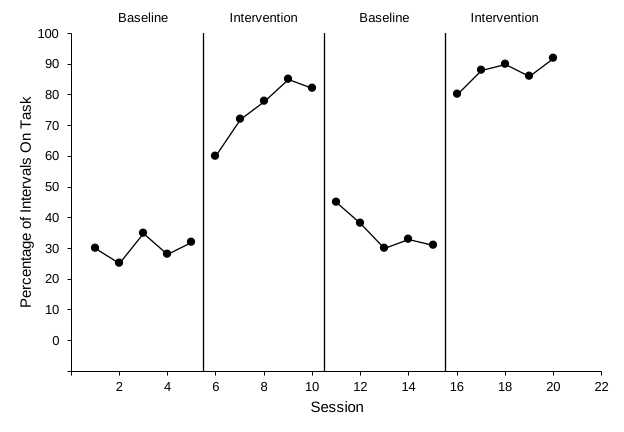
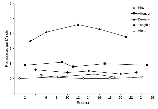
Before you move on, take a quick look at the chart. With the practice data:
- Each phase is its own path. No data line crosses a phase-change line.
- You can count three solid phase-change lines, at 5.5, 10.5, and 15.5 on the session axis, from the bottom of the plot area to the top.
- Five dashed criterion lines sit at 12, 20, 16, 26, and 30, and each spans only its own phase.
- Each condition is one continuous path, and no path drops to zero at sessions where that condition was not run.
- Every condition has its own marker: Baseline 1 filled circles, Intervention 1 filled circles, Baseline 2 filled circles, and Intervention 2 filled circles.
- The legend sits inside the plot area with no border and lists only Treatment A and Treatment B.
- There are no phase-change lines and no phase labels.
- The phase labels Baseline, Intervention, Baseline, and Intervention sit above the plot area, centered over their phases.are centered over their phases, on the top edge of the plot, as in Excel Lesson 4. The full figure makes room above them.
- The lowest vertical label is 0, one tick above the horizontal axis, and no negative label shows.
AI output varies. The same prompt can give slightly different results from one day to the next, or between Claude and ChatGPT. Never submit an AI-built graph without checking it. Use the audit prompt and checklist in the next lesson. You are responsible for the figure, just as you would be if you had built it yourself.
Adapting the prompt
- A different graph type: pick it at the top of the page. The prompt, the practice data link, and the target picture change to match.
- Different measure: change the vertical axis maximum, major unit, minimum (always minus one major unit), and title. End the vertical axis at 100 for percentages; for other measures, at a tick mark comfortably above your highest value, leaving room for a legend if there is one. The practice data are percentages, so the axis ends at 100. The practice rates peak at 2.5 responses per minute, and the axis ends at 3. The practice rates peak at 3.6 responses per minute, and the axis ends at 5, which leaves room for the legend and keeps low rates from being stretched to look like large differences. The practice data peak at 31 minutes, and the axis ends at 40. Keep the axis numbers whole: for rates, use a major unit of 1 or more rather than 0.5.
- Longer studies: change the horizontal major unit to 5 or 10, and set the horizontal maximum to the first multiple of that unit after your last session.
- More phases: for an ABC design or a longer reversal such as ABABAB, list every phase column in THE DATA and every label in step 10, in order.
- More phases: this prompt draws one phase-change line. For an ABC or ABAB design, pick Reversal (ABAB) at the top of the page. Its prompt draws a line at every phase change; list every phase column in THE DATA and every label in step 10, in order.
- All three tiers: use Lesson 4. Its recommended route, a template plus AI, keeps the tiers aligned for you.
- More treatments: add a column for each treatment, list it in THE DATA, give it its own marker in step 8, and add it to the legend in step 13.
- Different conditions: list your conditions in THE DATA, give each one a marker in step 8 that still reads clearly in black and white, and list them in the legend in step 10.
- Different criteria: change the criteria in THE DATA and the labels in step 12. For more or fewer criterion phases, also list every phase column in THE DATA.
- Shorter prompts: the prompt library has a compact AB and reversal promptthe prompt library has a compact alternating treatments promptthe prompt library has a compact multielement promptthe prompt library has a compact changing criterion promptthe multiple baseline prompts are in Lesson 4, not in the prompt library that relies on a shared style block.