

Overview › Build it in Excel › Lesson 1
Set up your data
The most important step in a single-case graph happens before you make the chart. If you put each phase in its own column, Excel breaks the data path at every phase change for you.
The most important step in a single-case graph happens before you make the chart. If you put each condition in its own column, Excel gives each condition its own data path, which is what lets a reader compare them.
You will be able to
- Set up a worksheet with session numbers in column A and one column per phasecondition, leaving the other cells empty, not 0.
- Explain why separate columns break the data path at each phase changegive each condition its own data path.
- Convert data kept in one long column into phasecondition columns with an
IFandNA()formula.
What you will build in this series
Across Lessons 1 to 4 you will turn a small table of numbers into this reversal (ABAB) design graph: the first tier, Participant 1, of a three-tier figure. Lessons 5 and 6 use the same skills for multiple baseline, alternating treatments, multielement, and changing criterion designs, so you can skip them for this graph. Lesson 5 copies this tier for Participants 2 and 3 and stacks the three tiers into one figure. Along the way you will connect each treatment's points across blank cells, give each condition its own marker, and add a legend. Lesson 6 recaps these settings for when you graph your own data. Along the way you will connect each condition's points across blank cells, give each condition its own marker, and add a legend. A multielement graph has no phase-change lines. Lesson 6 recaps these settings for when you graph your own data. Along the way you will add a dashed criterion line for each subphase and label each subphase with its criterion. Lesson 6 recaps these settings for when you graph your own data.
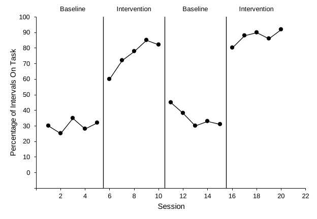
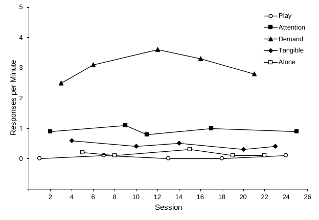
Want to follow along with the same numbers? Download practice-reversal-data.xlsx. It has the data already typed and nothing else. It holds all three participants. Lessons 1 to 4 use only Participant 1, in columns A:C.
The layout: one column per phasecondition
Put session numbers in column A. Give each phase its own column. Then type each session's value only in the column for the phase it belongs to, and leave the other cells in that row empty.
Put session numbers in column A. Give each condition its own column. Then type each session's value only in the column for the condition run in that session, and leave the other cells in that row empty.
| A | B | C | D | E | |
|---|---|---|---|---|---|
| 1 | Session | Baseline 1 | Intervention 1 | Baseline 2 | Intervention 2 |
| 2 | 1 | 30 | |||
| 3 | 2 | 25 | |||
| 4 | 3 | 35 | |||
| 5 | 4 | 28 | |||
| 6 | 5 | 32 | |||
| 7 | 6 | 60 | |||
| 8 | 7 | 72 | |||
| 9 | 8 | 78 | |||
| 10 | 9 | 85 | |||
| 11 | 10 | 82 | |||
| 12 | 11 | 45 | |||
| 13 | 12 | 38 | |||
| 14 | 13 | 30 | |||
| 15 | 14 | 33 | |||
| 16 | 15 | 31 | |||
| 17 | 16 | 80 | |||
| 18 | 17 | 88 | |||
| 19 | 18 | 90 | |||
| 20 | 19 | 86 | |||
| 21 | 20 | 92 |
Why separate columns? Excel draws one connected line for each column (each series). With four phase columns you get four separate data paths. That is exactly the break that single-case conventions require at each phase change. If all the values were in one column, Excel would join the last baseline point to the first intervention point. That suggests continuity between conditions that didn't happen (see Lesson 2).
In a multiple baseline design every tier follows the same rule, with its own Baseline and Intervention columns. Lessons 1 to 4 use only Participant 1's columns, A:C. In the practice file, columns D:G hold Participants 2 and 3; Lesson 5 uses them to build the other tiers.
Why separate columns? Excel draws one line for each column (each series), so each condition gets its own data path and, later, its own marker. That is what lets a reader compare the conditions session by session. Because the treatmentsconditions take turns, each treatment'scondition's column has blank cells between its values. In Lesson 3 you tell Excel to connect each condition's points across those blanks, so every condition reads as one continuous path. If all the values were in one column, Excel would draw a single zigzag line through every condition, and no reader could tell them apart.
The Baseline column has no values after session 4, so its path still ends at the phase change.
A multielement graph has no phase changes, so there are no breaks to make. The columns only keep the conditions apart.
Steps
- Open a blank workbook. WindowsOpen Excel and select Blank workbook, or press Ctrl+N if Excel is already open. MacOpen Excel and choose Blank Workbook, or press ⌘+N if Excel is already open.
- Type the column headings in row 1. In A1 type Session. In B1 to E1 type one heading per phasecondition: Baseline 1, Intervention 1, Baseline 2, and Intervention 2. Number repeated phases so each heading is unique. If a phase repeats in your own study, number the repeats (Baseline 1, Baseline 2) so each heading is unique. Number the criterion subphases so each heading is unique. Each condition keeps one column for the whole study, however many times it is run. You will type the labels shown on the graph separately in Lesson 4. You will type the phase labels shown on the graph separately in Lesson 4. The legend, though, uses these headings exactly as typed, so spell Treatment A and Treatment B the way you want them to appear on the graph. Excel uses these headings as the series names, and the legend you add in Lesson 4 lists them exactly as typed. Spell each condition the way you want it to appear on the graph. The P1 marks Participant 1; Participants 2 and 3 use P2 and P3 in columns D to G.
- Number the sessions in column A. Type 1 in A2 and 2 in A3. Select both cells, then drag the small square at the bottom-right corner of the selection (the fill handle) down until the last session number appears: 20 in A21.
- Type each value in its phase'scondition's column. Sessions 1 to 5 go in column B, sessions 6 to 10 in column C, and so on. Sessions 1 to 5 go in column B and sessions 6 to 15 in column C. Sessions 1 to 5 go in column B and sessions 6 to 18 in column C. Sessions 1 to 5 go in column B, sessions 6 to 8 in column C, sessions 9 to 13 in column D, and so on. Each criterion subphase gets the next column. Sessions 1 to 4 (baseline) go in column B. After that, each session's value goes in the column of the treatment run that session: session 5 in column C (Treatment A), sessions 6 and 7 in column D (Treatment B), sessions 8 and 9 back in column C, and so on. Each session's value goes in the column of the condition run that session: session 1 in column B (Play), session 2 in column C (Attention), session 3 in column D (Demand), and so on. Each row should have a value in exactly one phasecondition column, B or C.
- Leave the other cells truly empty. Don't type 0, a space, or a dash in cells that belong to other phasesconditions. Excel would plot a 0, or treat the column as text. If you typed something by mistake, select the cell and press Delete. A real zero is different: if you measured the behavior in a session and it was zero, type 0 in that session's own column so the point is plotted. In the practice data, Play is 0 in sessions 1, 13, and 18.
- Save the workbook.
WindowsPress Ctrl+S and save as an Excel Workbook (
.xlsx). MacPress ⌘+S and save as an Excel Workbook (.xlsx).
If your data are already in one long column
Data sheets often have three columns: Session, PhaseCondition, and Value. You don't have to retype anything. Add one column per phasecondition with a formula that copies the value only when the phasecondition matches. For example, if the phasecondition name is in column B and the value is in column C, put this in the Baseline 1 column and fill it down:
=IF($B2="Baseline 1", $C2, NA())
In each of the other new columns, change the name in quotes to that column's heading. Use NA(), not "". Excel plots an empty-looking "" as 0 in this kind of chart, but it skips #N/A. The #N/A cells look untidy in the sheet. You can hide them with conditional formatting, or just leave them, because they never print on the graph. When you connect each condition's points across blank cells in Lesson 3, Excel joins them across these #N/A cells too.
The name in quotes must match what your Phase column says. Many data sheets repeat the same names: Baseline, Intervention, Baseline, Intervention. Then the formula can't tell the first baseline from the second. "Baseline 1" matches nothing and fills its column with #N/A, and "Baseline" puts both baselines in one column. Fix it one of two ways:
- Number the runs in your Phase column itself (Baseline 1, Intervention 1, Baseline 2, Intervention 2), so each name matches one heading.
- Number the runs in a new column instead, right after Value and before the phase columns. In D1 type Run, in D2 type
=IF(B2=B1, D1, N(D1)+1), and fill it down. Each time the phase name changes, the number goes up by 1, so the four phases get 1, 2, 3, and 4 in order. Then match on that number instead of the name:=IF($D2=1, $C2, NA())in the Baseline 1 column,=IF($D2=2, $C2, NA())in the Intervention 1 column, and so on. When you delete the Phase and Value columns (next paragraph), delete the Run column too.
The name in quotes must match what your Phase column says, so each subphase needs its own name there. If your data sheet uses one name for more than one subphase, such as Intervention for every criterion level, rename the subphases in your Phase column first (Phase 1, Phase 2, and so on), so each name matches one heading.
Later lessons expect Session in column A and the phasecondition columns right after it, starting in column B. Once the formulas are filled down, select the new columns, copy them, and paste them back over themselves as values: Home›Paste›Paste Special, choose Values, and click OK. Then select the original PhaseCondition and Value columns and choose Home›Delete›Delete Sheet Columns. Paste the values first; deleting those columns while the formulas still point at them turns every result into #REF!.
Shortcut with AI. The Claude and ChatGPT add-ins can restructure long data into phasecondition columns for you. See the restructure prompt in the prompt library (AI Lesson 5).
Check before moving on
- Column A holds session numbers that run 1, 2, 3 … 20 without gaps or text
- Each phasecondition has its own column, with a unique heading in row 1 (B1:E1)
- Each row has a value in exactly one phasecondition column, B or C
- Cells for other phasesconditions are empty, not 0
- Each treatment'scondition's column has blank cells between its values. That is expected; Lesson 3 connects the points
- For Lessons 2 to 4 you use only columns A:C, Participant 1's data