

Overview › Build it in Excel › Lesson 5
Multiple baseline graphs
A multiple baseline figure is a stack of identical graphs, one per participant, behavior, or setting. They share one horizontal axis and are joined by a stepped phase-change line. You built the top tier in Lessons 1 to 4. Here you make it short, copy it, point each copy at its own data, and line the tiers up.
You will be able to
- Make a short tier, copy it for each participant, and point each copy at its own data and its own phase-change line.
- Stack and align the tiers so their plot areas line up, with phase labels above the top tier only and one vertical axis title.
- Draw the stepped line that joins the phase changes across tiers, and group the figure.
Not needed for your graph. This lesson is only for multiple baseline graphs, and your graph type is set to Reversal (ABAB). Your graph is complete after Lesson 4, so go on to Lesson 7: Export and place the figure.Go on to Lesson 6: Alternating treatments, multielement, and changing criterion. To build a multiple baseline graph instead, switch to Multiple baseline.
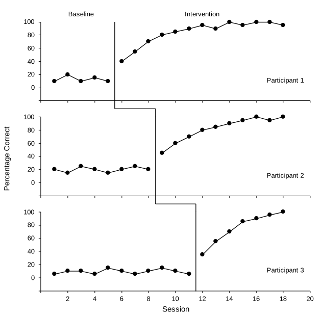
Practice data: practice-multiple-baseline-data.xlsx. It holds all three tiers. Lessons 1 to 4 used Participant 1 in columns A:C. This lesson adds the other two.
Part A: Check the data layout
The practice workbook uses one Session column and two columns per tier, one for Baseline and one for Intervention. This is Lesson 1's rule applied to each tier. Participant 1 is in columns B and C, Participant 2 in D and E, and Participant 3 in F and G.
| A | B | C | D | E | F | G | |
|---|---|---|---|---|---|---|---|
| 1 | Session | P1 Baseline | P1 Intervention | P2 Baseline | P2 Intervention | P3 Baseline | P3 Intervention |
| 2 | 1 | 10 | 20 | 5 | |||
| 3 | 2 | 20 | 15 | 10 | |||
| 4 | 3 | 10 | 25 | 10 | |||
| 5 | 4 | 15 | 20 | 5 | |||
| 6 | 5 | 10 | 15 | 15 | |||
| 7 | 6 | 40 | 20 | 10 | |||
| 8 | 7 | 55 | 25 | 5 | |||
| 9 | 8 | 70 | 20 | 10 | |||
| 10 | 9 | 80 | 45 | 15 | |||
| 11 | 10 | 85 | 60 | 10 | |||
| 12 | 11 | 90 | 70 | 5 | |||
| 13 | 12 | 95 | 80 | 35 | |||
| 14 | 13 | 90 | 85 | 55 | |||
| 15 | 14 | 100 | 90 | 70 | |||
| 16 | 15 | 95 | 95 | 85 | |||
| 17 | 16 | 100 | 100 | 90 | |||
| 18 | 17 | 100 | 95 | 95 | |||
| 19 | 18 | 95 | 100 | 100 |
Keep the helper tables clear of columns D to G. Tiers 2 and 3 need those columns, so the phase-change line and label tables from Lesson 4 must sit to the right of column G. Look at where you typed them. If either one is anywhere in columns D to G, move it now: select the whole table, point to the edge of the selection until the pointer changes, and drag the table to empty columns to the right of everything else, keeping it in the same rows. Leave at least four empty rows below the phase-change line table, because Part C adds four rows to it. The chart's series follow cells you move. Then check that tier 1's phase-change line is still in place and its labels still read Baseline and Intervention. If the labels changed, redo the Value From Cells step from Lesson 4. Finally, if a table covered any of Participant 2's or 3's cells, open a fresh download of the practice file, copy D1:G19, and paste it into cell D1 of your sheet.
Part B: Make the top tier short
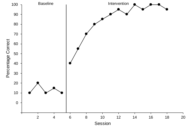
- Start from your tier 1 chart. Lessons 1 to 4, with Multiple baseline chosen in the Graph box, built Participant 1 (columns A:C) as a finished graph: black axes, a floating zero, axis titles, a phase-change line after session 5, and the labels Baseline and Intervention. Every tier will be a copy of this chart, so fix anything in it now. If you haven't built it yet, start at Lesson 1.
- Make it short and wide. Select the chart. On the Format tab, set Width to 6.5" and Height to 2" (16.51 cm and 5.08 cm). Three tiers of about 2 inches each fit on one page with room for the figure number, title, and note.
- Rescale the vertical axis for a short tier. A 2-inch tier has no room for a label every 10. Double-click the vertical axis numbers. In Format Axis › Axis Options, set Minimum to -20 and Major to 20, and leave Maximum at 100. Under Horizontal axis crosses, change Axis value to -20. The format code 0;;0 from Lesson 3 already hides the −20 label, so zero still floats one tick above the horizontal axis. Then, in your phase-line helper table from Lesson 4, change the bottom Line Y value (row 2, cell K2 if the table starts in J1 as Lesson 4 placed it) from -10 to -20 so the line still reaches the horizontal axis. Every tier will copy these bounds, and every tier keeps the same horizontal axis, 0 to 20.
- Hide the session numbers on this tier. Double-click the horizontal axis numbers. In Format Axis, expand Labels and set Label Position to None. Keep the axis line and tick marks. Then click this tier's horizontal axis title, Session, and press Delete.
- Blank the vertical axis title, but keep it. Click the vertical axis title, Percentage Correct, select its text, and replace it with a single space. The tier then reserves the same left margin as the middle tier, which will carry the real title. That keeps every plot area lined up.
- Add the tier name. With the chart selected, insert a text box (Insert›Text›Text BoxInsert›Text Box). Click inside the plot near the bottom-right corner and type Participant 1, in Arial 10 pt.
Part C: Copy the tier and point each copy at its own data
Each tier gets its own phase-change line, drawn from its own two rows of the phase-line helper table you made in Lesson 4. Tier 1 already uses rows 2 and 3. Tiers 2 and 3 go in the rows directly below:
| Tier | Helper table rows | Cells (X values / Y values) | Line X | Line Y |
|---|---|---|---|---|
| Tier 1 (Participant 1) | 2 and 3, from Lesson 4 | J2:J3 / K2:K3 | 5.5 and 5.5 | −20 and 100 |
| Tier 2 (Participant 2) | 4 and 5 | J4:J5 / K4:K5 | 8.5 and 8.5 | −20 and 100 |
| Tier 3 (Participant 3) | 6 and 7 | J6:J7 / K6:K7 | 11.5 and 11.5 | −20 and 100 |
Each line sits halfway between a tier's last baseline session and its first intervention session. The cells assume the table starts in J1, where Lesson 4 put it for the multiple baseline practice file; if you moved it, use the same rows in your columns. The phase-label table stays as it is, because only the top tier has phase labels.
- Copy the chart twice. Click the chart's edge and press Ctrl+C. Click an empty cell below the chart and press Ctrl+V. Click another empty cell and paste again. ⌘+C. Click an empty cell below the chart and press ⌘+V. Click another empty cell and paste again.
- Type the new helper rows. In rows 4 to 7 of the phase-line helper table, type the tier 2 and tier 3 values from the table above: 8.5, 8.5, 11.5, and 11.5 under Line X, and -20, 100, -20, and 100 under Line Y. Do this before you open Select Data, because Excel won't let you type in cells while that dialog is open.
- Repoint tier 2's data paths. Click the second chart and open Chart Design›Select Data. Select the baseline series, P1 Baseline, the first one in the list. Click Edit. Change Series name to cell D1 and Series Y values to D2:D19: click in each box, delete what is there, and select the cells on the sheet. Click OK.Its boxes appear on the right. Change Name to cell D1 and Y values to D2:D19: click in each box, delete what is there, and select the cells on the sheet. Do the same for the intervention series, P1 Intervention, using E1 and E2:E19. The X values stay on A2:A19.
- Give tier 2 its own phase-change line. Still in Select Data, select the Phase change series and click Edit. Point its X values at the Line X cells in rows 4 and 5 (J4:J5) and its Y values at the Line Y cells in rows 4 and 5 (K4:K5). Click OK.
- Remove the phase labels from tier 2. In Select Data, select the Phase labels series and click Remove−. Label phases on the top tier only. Click OK to close Select Data.
- Type the real vertical axis title on tier 2. Tier 2 is the middle tier. Replace its blank title with Percentage Correct, so one title serves the whole figure and sits near its middle. Change its tier name to Participant 2.
- Set up tier 3 the same way. Use columns F and G (F1 and F2:F19, G1 and G2:G19), the phase-change rows 6 and 7 of the helper table (J6:J7 and K6:K7), and the tier name Participant 3. Remove its phase labels and leave its vertical title blank. Then:
- turn its session numbers back on (Labels › Label Position › Next to Axis)
- add the horizontal axis title back (Chart Design›Add Chart Element›Axis Titles›Primary Horizontal), type Session, and set it to Arial 11 pt, black, like the vertical title
- make it about 0.4" taller than the other tiers (2.4", or 6.1 cm) to make room for the numbers and title
Part D: Stack and align the tiers
- Make room above tier 1’s phase labels. Click tier 1’s edge. On the Format tab, change Height from 2" to 2.2" (5.59 cm). Excel makes its plot area about 0.2 in taller. Then click an empty spot inside tier 1’s plot area, away from the points and lines, and drag the handle in the middle of its top edge down about 0.2 in (0.5 cm). When you let go, Baseline and Intervention sit just above the plot area, with a small gap below them. Tier 1’s plot area is then the same height as tier 2’s, and the extra 0.2 in is all above it, holding the labels.
- Select all three charts. WindowsClick the first chart's edge, then hold Ctrl and click the edges of the other two. MacClick the first chart's edge, then hold Shift and click the edges of the other two.
- Align their left edges. On the Format tab (Shape Format in some versions), choose Align›Align Left.
- Stack them closely. Drag tier 2 up until its top edge just touches the bottom of tier 1, then drag tier 3 up under tier 2. Overlapping the empty chart edges slightly is fine.
- Check the vertical axes form one straight column. Every tier has the same width, the same tick labels, and a vertical title (blank or real). So the plot areas should line up exactly. If one is off, click that tier's plot area (inside the axes) and drag its left handle to match the tiers above. Also check that the plot areas are the same height, measured from the horizontal axis to 100, so every tier shows the same vertical scale. Drag a plot area's top or bottom handle to fix one that differs.
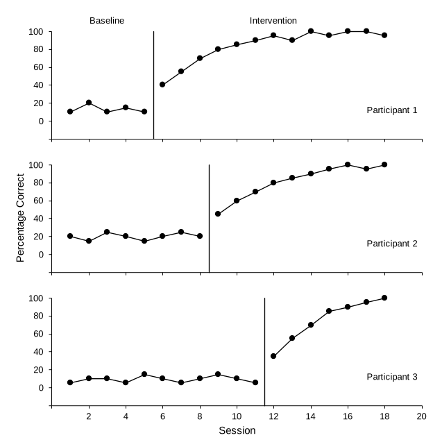
Part E: Draw the stepped phase-change line
The short segments that join the tiers sit in the gaps between charts, so they are drawn shapes on the worksheet.
- Click an empty cell first. That way the lines are drawn on the worksheet, not inside one of the charts.
- Zoom in. Use the zoom slider at the bottom-right of the window to work at 150–200%.
- Draw three segments for each step.
Choose Insert›Illustrations›Shapes›LineInsert›Shapes›Line. Hold Shift while dragging to keep each line perfectly straight. Draw:
- down from the bottom of tier 1's phase-change line to halfway into the gap
- across to directly above tier 2's phase-change line
- down to the top of tier 2's phase-change line
- Format the segments. Click one segment, then hold Shift and click the other five. On the Shape Format tab, set Shape Outline to black and its Weight to 1 pt, the same as the phase-change lines. Use the arrow keys to nudge a segment until its ends meet the chart's phase-change lines.
Part F: Group everything
- Select the charts and the six segments. WindowsGo to Home›Find & Select›Select Objects, then drag a box around the whole figure. Press Esc afterward to leave this mode. MacClick the first chart's edge, then hold Shift and click each other chart and each segment.
- Group them. Right-click any selected object and choose Group›Group. Control-click any selected object and choose Group›Group. The figure now moves, copies, and exports as one picture. To edit one tier later, click the figure once, then click the tier.
Shortcut: The multiple baseline template does Parts B to F for you. Type your data and each tier's phase-change line moves automatically. Only the six connector segments need nudging if your phase timing differs from the example.
Across participants, behaviors, or settings? The figure is built the same way. Only the tier names change (for example, Home, School, Clinic). More than three tiers? Copy a middle tier again, give it two new rows in the phase-line helper table, and move the real vertical title to the tier nearest the middle.
Check before moving on
- Every tier has the same axes: horizontal 0 to 20, vertical −20 to 100 in steps of 20, with the −20 label hidden so zero floats above the horizontal axis
- Each tier plots its own Baseline and Intervention columns against the sessions in column A
- Each tier's phase-change line falls between its last baseline and first intervention session (5.5, 8.5, and 11.5) and runs the full height of the plot
- Phase labels appear above the top tier’s plot area only (tier 1 is 2.2 in tall, with the extra 0.2 in above its plot area), and each tier has its name inside the plot
- One vertical axis title, on the middle tier; session numbers and the Session title on the bottom tier only
- Every tier is 6.5 in wide, and the plot areas line up on the left and are the same height
- The six connector segments are black, 1 pt, and meet each tier's phase-change line with no gaps, and the charts and segments are grouped