

Overview › Build it in Excel › Lesson 3
Format for APA style
Strip out Excel's decoration, then set up the axes, data paths, fonts, and axis titles. Each part below ends with a picture of how your chart should look. You are formatting the Participant 1 chart. Lesson 5 copies it for the other tiers, so every setting you make here carries over. For your graph, Part E also joins each condition's points across blank cells and gives each condition its own marker.
You will be able to
- Remove Excel’s chart title, legend, gridlines, and border, and set one sans serif font for the whole chart.
- Set the bounds and units of both axes, with zero floating one tick above the horizontal axis, and work them out for new data in the practice.
- Make every data path black with filled circle markers and continuous across blank cells, with a different marker for each condition, and add axis titles that name the measure.
The Format pane is your main tool. Almost every setting in this lesson lives in the Format pane that opens on the right side of the window. Open it by double-clicking any part of the chart, or by right-clicking the part and choosing Format …. You can also select the part and press Ctrl+1. Open it by double-clicking any part of the chart, or by Control-clicking the part and choosing Format …. You can also select the part and press ⌘+1. The pane stays open. When you click another part of the chart, the pane switches to that part.
Part A: Remove the title, legend, and gridlines
- Turn off the three extras. WindowsClick the chart. Click the + (Chart Elements) button that appears beside its top-right corner. Uncheck Chart Title, Gridlines, and Legend. MacClick the chart, then go to Chart Design›Add Chart Element. Choose Chart Title›None, then Legend›None. Then open Gridlines and click each checked gridline option to turn it off. On either system you can also click the title, the legend, or a gridline and press Delete. Remove the legend now even though your graph needs one. Excel's default legend lists every column and has a border. You add a small, borderless legend back in Lesson 4, once every condition has its final marker.
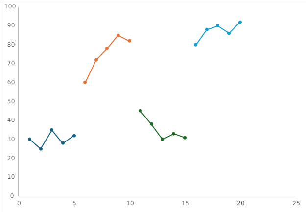
Part B: Remove the border and set the font
- Remove the chart border. WindowsRight-click an empty area near the chart's edge and choose Format Chart Area. MacControl-click an empty area near the chart's edge and choose Format Chart Area. In the pane, click the Fill & Line icon (the paint bucket). Under Border, choose No line. Leave Fill as a white solid fill.
- Set one font for the whole chart. With the chart area still selected (click the chart's edge if not), go to the Home tab. Set the font to Arial, size 10, and the font color to black (Automatic or Black). Every label in the chart changes at once.
Why Arial? APA style asks for a sans serif font in figures, between 8 and 14 points. Arial is installed on every Windows and Mac computer, so the chart looks the same on a coauthor's machine. Calibri and Helvetica are also fine. Whatever you choose, use the same font in every figure.
Part C: Format the vertical axis
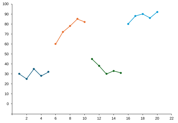
- Open Format Axis for the vertical axis. Double-click the numbers along the vertical axis. The Format Axis pane opens with Axis Options (the bar-chart icon) selected.
- Set the bounds and units. Under Bounds, type -10 in Minimum and 100 in Maximum. Under Units, type 10 in Major. Press EnterReturn after each value. The word Auto changes to a Reset button, which means your value is locked in. For your own data, end the vertical axis at 100 for percentages; for other measures, at a tick mark comfortably above your highest value, leaving room for a legend if your graph has one. Phase labels go above the plot area, so they need no room inside it. The practice data are percentages, so the maximum is 100. The practice rates peak at 2.5, so a maximum of 3 leaves room for the legend you add in Lesson 4. The practice rates peak at 3.6, so a maximum of 5 leaves room for the legend you add in Lesson 4. The practice data peak at 31 minutes, so a maximum of 40 keeps the highest point well below the top of the plot.
- Drop the horizontal axis below zero. In the same section, under Horizontal axis crosses, choose Axis value and type -10. The horizontal axis moves to the bottom, and 0 now sits one tick above it. This number always matches the Minimum. Excel doesn’t update it for you, so if you change the Minimum later, change this box too. Otherwise the horizontal axis sits above the bottom tick.
- Hide the negative label. Expand Number. In Format Code, type 0;;0 and click Add. The "-10" disappears, but its tick mark stays at the corner where the axes meet. Your graph shows a rate, but its axis still counts in whole numbers (0, 1, 2, and so on), so the same code works. The empty middle part of the code is what hides negative numbers.
- Put the tick marks outside. Scroll down in the same pane and expand Tick Marks. Set Major type to Outside and Minor type to None.
- Make the axis line black. Click the Fill & Line icon at the top of the pane. Under Line, choose Solid line, set Color to black, and set Width to 0.75 pt.
Why a floating zero? If 0 sits right on the horizontal axis, data points at zero merge with the axis line and are hard to see. Behavior-analytic journals have long placed zero slightly above the horizontal axis. The graphs drawn elsewhere on this site raise it by half a major unit. Excel can’t: it always starts its tick marks at the axis minimum, so on a 0 to 100 scale a minimum of −5 with a major unit of 10 labels the ticks 5, 15, 25 instead of 0, 10, 20. In Excel the minimum has to be exactly one whole major unit below zero. Here that is -10 with a major unit of 10.
Axis Options
Bounds
Units
Horizontal axis crosses
Tick Marks
Labels
Number
Part D: Format the horizontal axis
- Select the horizontal axis. With the pane still open, click the numbers under the horizontal axis. The pane switches to that axis.
- Set the bounds and units. Set Minimum to 0 and Major to 2. For Maximum, use one more than your last session, so the last point is not squeezed against the edge of the plot. If that number falls between two tick marks, round up to the next tick. The practice data end at session 20, and one more falls between two ticks, so type 22. For your own data, use a major unit of 1 with 10 or fewer sessions, and 5 or 10 with more than 40.
- Match the vertical axis. Set Tick Marks › Major type to Outside. Then, under Fill & Line, set the line to Solid line, black, 0.75 pt. Leave Vertical axis crosses on Automatic so the two axes meet at 0.
- Hide session 0. There is no session 0, so hide that label. Under Number, type the format code 0;; and click Add. The tick mark stays and the "0" disappears.
- Keep the axis numbers whole. For rates such as responses per minute, count the vertical axis in whole numbers too: a major unit of 1 (or 2, 5, 10…), not 0.5, so the labels read 0, 1, 2 rather than 0.0, 0.5, 1.0. Use the matching floating zero, a minimum of -1, set Horizontal axis crosses › Axis value to -1 as well, and keep the format code 0;;0. The points still plot at their exact rates. Your graph shows a rate, but Part C still counted the vertical axis in whole numbers: a major unit of 1, a minimum of -1, and the format code 0;;0. The points still plot at their exact rates, such as 0.6 or 2.5; only the axis numbers are whole. Keep the horizontal axis in whole sessions too.
Part E: Make every data path black
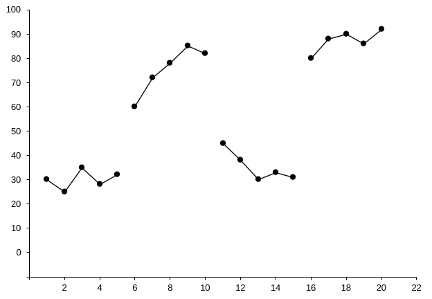
- Connect each condition across its blank cells. Each condition's column is blank wherever another condition ran, and Excel leaves a gap at every blank cell, so a condition's points are not joined. Click the chart and open Chart Design›Select Data. WindowsIn the Select Data Source box, click Hidden and Empty Cells at the bottom-left and choose Connect data points with line. Click OK twice. MacIn the Hidden and Empty Cells area at the bottom of the Select Data Source box, set Show empty cells as to Connect data points with line. Click OK. Each condition is now one continuous path. The Baseline path still ends at the phase change, because its column has no values after session 4.
- Select the first data path. Click once on any point of the Baseline 1 path. All of its points should show selection handles. The pane switches to Format Data Series.
- Format the line. Click Fill & Line (paint bucket), then Line at the top of that section. Choose Solid line, color black, width 1 pt.
- Format the markers. Click Marker (next to Line). Under Marker Options choose Built-in, type ● (circle), size 6. Under Fill choose Solid fill, black. Under Border choose Solid line, black.
- Give the condition its own marker. Click Marker (next to Line). Under Marker Options choose Built-in, pick the shape from the Type list (it shows pictures of the shapes), and set size 6. Use one shape and fill per condition: Baseline filled circles, Treatment A filled squares, and Treatment B open triangles. For a filled marker, set Fill to Solid fill, black. For an open marker, set Fill to Solid fill, white, so the line does not show through it. Either way, set Border to Solid line, black.
- Repeat for each phasecondition. Click the next data path. The pane stays open, so you only need to repeat the line and marker settings. Use the same settings for every phase of the same condition. Keep every line and marker border black. Only the marker shape and fill change from one condition to the next.
Part F: Add axis titles
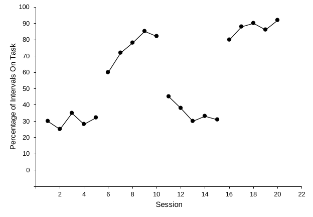
- Turn on axis titles. WindowsClick the chart, click + (Chart Elements), and check Axis Titles. MacGo to Chart Design›Add Chart Element›Axis Titles›Primary Horizontal. Then repeat and choose Primary Vertical.
- Type the titles. Click the placeholder text Axis Title under the horizontal axis. Select the text and type Session. Do the same for the vertical title. For the practice data, type Percentage of Intervals On Task. Excel rotates the vertical title for you.
- Check the title font. Axis titles may have come in larger or bold. Select each title and set it to Arial, 11 pt, not bold, black.
Check before moving on
- No chart title, legend, gridlines, or chart borderNo chart title, gridlines, or chart border, and no legend yet
- All text is Arial (or one other sans serif font), black, 10–11 pt
- Vertical axis -10 to 100 in steps of 10, with the -10 label hidden, so zero floats above the horizontal axis
- The vertical axis’s Horizontal axis crosses › Axis value is also -10, so the horizontal axis meets the bottom tick
- Vertical axis labels are whole numbers (format code 0;;0)
- Horizontal axis 0 to 22 in steps of 2, with the 0 label hidden
- Chart 6.5 × 4.5 in, so the plot area is about 2:3
- Both axes are solid black lines with outside tick marks
- Every data path is a black line with black circle markersEach condition is one continuous black path across its blank cells, with its own marker: Baseline filled circles, Treatment A filled squares, and Treatment B open triangles
- Both axis titles are present and in title case: Session and Percentage of Intervals On Task
Practice: set up the axes
Work out the floating-zero minimum, the horizontal axis maximum, and, as a preview of Lesson 4, where phase-change lines go. New questions appear each time.
Save your formatting as a chart template. Once a chart looks right, you can reuse the look. Right-click the chart and choose Save as Template. Later, choose Insert›Recommended Charts›All Charts›Templates. Control-click the chart and choose Save as Template. Later, choose Chart Design›Change Chart Type›Templates. A chart template keeps fonts, colors, and axis styling, but not phase-change lines or labels. For a fully reusable graph, use the workbook templates.