
Overview › Build it in Excel › Lesson 2
Create the graph
Insert an X Y (scatter) chart with straight lines and markers, check that Excel read your columns correctly, and set the chart to its final printed size.
You will be able to
- Build a scatter chart with straight lines and markers that uses the session numbers in column A as its x-values, and fix one that doesn’t.
- Explain why a single-case graph uses a scatter chart, not a line chart.
- Set the chart to its final printed size before you format it.
Why a scatter chart and not a line chart? A line chart treats the session numbers as text labels. It spaces them evenly whether or not sessions are missing, and it gives you no number for the position between sessions. A scatter chart places every point at its real session number. That lets you put a phase-change line exactly at session 5.5, and it lets you control the axis range precisely.That keeps each condition's points at the sessions when they actually ran, and it lets you control the axis range precisely. The chart subtype with straight lines and markers gives the familiar single-case look.
Steps
- Select the data, including the headings. Click cell A1 and drag across to the last phase columnParticipant 1's last phase columnthe last condition column and down to the last row of data (E21 in practice-reversal-data.xlsx), so the selection is A1:E21. You can also click A1 and then Shift-clickShift-click E21. That last cell is empty, because the final session in the practice data wasn't an Alone session. Include it anyway, so the selection covers every session. That selects only the Session column and Participant 1's two columns. The practice file also holds Participants 2 and 3 in the columns to the right. Leave them out for now: this lesson and the next two build Participant 1's tier as a full-size chart, and Lesson 5 adds the other tiers.
- Insert a scatter chart with straight lines and markers. WindowsGo to Insert›Charts group›Insert Scatter (X, Y) or Bubble Chart. This is the button with a dot-plot icon. Then choose Scatter with Straight Lines and Markers, the fourth icon in the Scatter row. Hover over an icon to see its name. MacGo to the Insert tab and click the X Y (Scatter) chart button (the dot-plot icon, tooltip Insert Scatter (X, Y) or Bubble Chart). Then choose Scatter with Straight Lines and Markers, the fourth icon in the Scatter row.
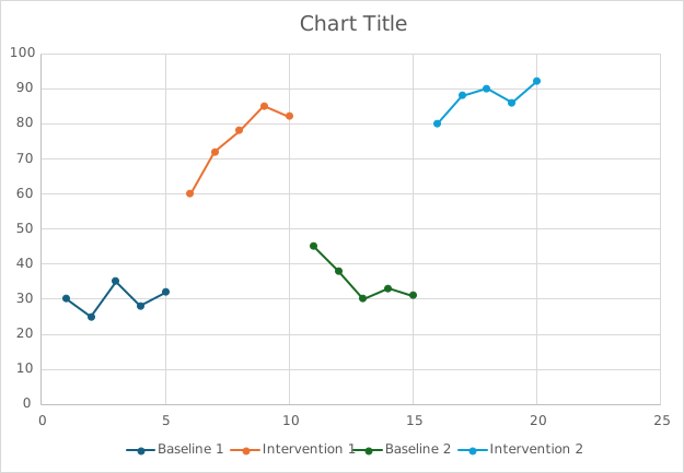
- Compare your chart with this picture. You should see four colored data paths with a gap at each phase change. There will also be a "Chart Title," gridlines, and a legend listing your four phase headings. Lesson 3 removes all of that. You should see four colors, one for each condition column: Baseline 1, Intervention 1, Baseline 2, and Intervention 2. The Baseline points are joined into one path, but Treatment A and Treatment B show only short pieces and lone points. Two points are joined only where the same treatment ran in back-to-back sessions. Every point stands alone, with no lines between them, because in the practice data no condition ran in back-to-back sessions. That is expected for now. Each condition's column has a blank cell for every session in which a different condition ran, and Excel leaves a gap at each blank cell. Lesson 3 connects each condition's points across those blanks. There will also be a "Chart Title," gridlines, and a legend listing your four condition headings. Lesson 3 removes all of that; a later lesson adds a cleaner legend back inside the graph.
Doesn't match? If one of the series is named Session, or the horizontal axis runs 1, 2, 3 … regardless of your data, Excel didn't read column A as the x-values. Click the chart and open Chart Design›Select Data. Under Legend Entries (Series), select Session and click Remove. Then select each remaining series and click Edit. In the Edit Series box, click in Series X values, delete what is there, drag over the session numbers in $A$2:$A$21, and click OK.Select Session in the Legend entries (Series) list and click the − button. Then select each remaining series; its boxes appear on the right. Click in X values, delete what is there, and drag over the session numbers in $A$2:$A$21. Excel adds the sheet name for you, for example =Data!$A$2:$A$21 in the practice file. When every series is done, click OK to close Select Data. If the axis still runs 1, 2, 3 …, some session numbers in column A are probably stored as text; retype them as plain numbers. The quickest fix is often to delete the chart, check that A1 contains the word Session, select the data again, and re-insert the chart.
- Move the chart off your data. Point at the chart's outer edge until the pointer becomes a four-headed arrow, then drag the chart below your data, so its top-left corner sits in column A a couple of rows under your last row of data (row 21 in the practice file). Keep the columns to the right of your data clear: Lesson 4 types small helper tables there. Keep the chart off the columns to the right of Participant 1's data: they hold Participants 2 and 3, and Lesson 4 types small helper tables to the right of those. That way the chart covers none of your cells.
- Set the final size now. WindowsWith the chart selected, go to the Format tab. In the Size group at the far right, set Height to 4.5" and Width to 6.5". MacWith the chart selected, go to the Format tab. In the height and width boxes at the right of the ribbon, set Height to 4.5" and Width to 6.5". If your Excel measures in centimeters, use 11.43 cm and 16.51 cm. For a multiple baseline graph, build Participant 1's tier at this full size for now. Lesson 5 makes each tier shorter and stacks the tiers.
Why size first? Font sizes are fixed in points. If you format a large chart and then shrink it when you paste it into Word, the 10-point text becomes unreadably small. APA asks for figure text between 8 and 14 points at final size. So build the chart at the size it will be printed. A 6.5-inch width fills a page with 1-inch margins. Many journals print single-column figures about 3.25 inches wide. Check your journal's guidelines.
Why 4.5 inches tall? Graphing standards recommend that the plot area (the space inside the axes) be about two-thirds as tall as it is wide. The accepted range is between 5:8 and 3:4. Flatter graphs make changes look smaller, and taller ones make them look bigger. At 6.5 × 4.5 inches, with the fonts used in these lessons, the plot area comes out close to 2:3. Lesson 4 lowers the top of the plot area about 0.2 in to make room for the phase labels above it. That brings it a little under 2:3, still inside the 5:8 to 3:4 range. If you change the size, check the plot area itself: hold a ruler to the screen at 100% zoom, or compare the axis lengths.
The most common mistake
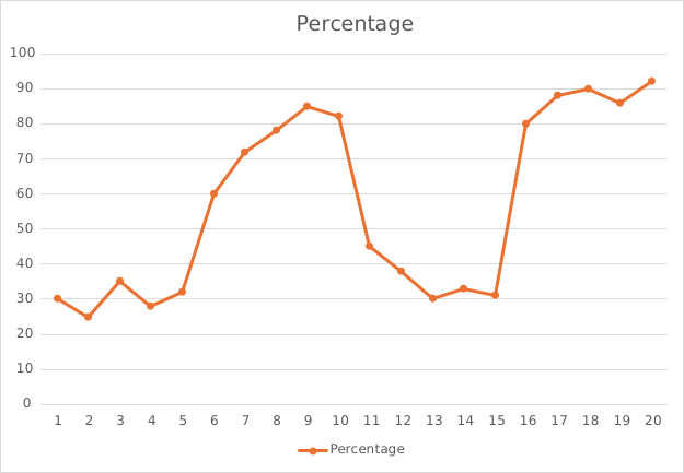
Here is the same datathe reversal (ABAB) practice data typed into a single column and plotted as a line chart. The path climbs straight from the last baseline point into intervention, so the phase change disappears into one continuous line. When conditions alternate, the result is worse: one zigzag line runs through every condition in session order, so no one can tell which point belongs to which condition. On the right is the chart from step 3, built the right way.